ARIMAX/SARIMAX/VAR

ARIMAX

ARIMAX model assumes that future values of a variable linearly depend on its past values, as well as on the values of past (stochastic) shocks. It is an extended version of the ARIMA model, with other independent (predictor) variables. The model is also referred to as the dynamic regression model. The X added to the end stands for “exogenous”. In other words, it suggests adding a separate different outside variable to help measure our endogenous variable.

The ‘exogenous’ variables added here are COVID-19 case numbers and COVID-19 vaccine rates. The number of COVID-19 cases in US can affect healthcare stock prices, e.g. UNH. Higher case numbers may result in increased demand for healthcare services, such as hospitalizations, treatments, and testing, which could positively impact the stock prices of healthcare companies involved in providing those services. Conversely, lower case numbers may lead to reduced demand for healthcare services, potentially resulting in lower stock prices for healthcare companies.

Vaccine rates, specifically the rate at which a population is vaccinated against COVID-19, can also impact healthcare stock prices. Higher vaccine rates are generally seen as positive for healthcare companies, as vaccines are considered a key tool in controlling the spread of the virus and reducing the severity of illness. Higher vaccine rates may lead to decreased demand for COVID-19 treatments and testing, but increased demand for vaccines and other preventive healthcare measures, which could positively impact the stock prices of healthcare companies involved in vaccine production or distribution, as well as other preventive healthcare services.

In this section, we choose the UNH stock price to fit ARIMAX model with COVID-19 case numbers and COVID-19 vaccine rates.

Step 1: Data Prepare

Show the code

getSymbols("UNH", from="2020-12-16", src="yahoo")

Show the code

UNH_df <- as.data.frame(UNH)
UNH_df$Date <- rownames(UNH_df)
UNH_df <- UNH_df[c('Date','UNH.Adjusted')]
UNH_df <- UNH_df %>%
  mutate(Date = as.Date(Date)) %>%
  complete(Date = seq.Date(min(Date), max(Date), by="day"))

# fill missing values in stock 
UNH_df <- UNH_df %>% fill(UNH.Adjusted)

new_dates <- seq(as.Date('2020-12-16'), as.Date('2023-3-21'),'week')

UNH_df <- UNH_df[which((UNH_df$Date) %in% new_dates),]

vaccine_df <- read.csv('data/vaccine_clean.csv')

new_dates <- seq(as.Date('2020-12-16'), as.Date('2023-3-22'),'week')

#vaccine_df
vaccine_df$Date <- as.Date(vaccine_df$Date)
vaccine_df <- vaccine_df[which((vaccine_df$Date) %in% new_dates),]

#covid_df
covid_df <- read.csv('data/covid.csv')

#covid_ts <- ts(covid_df$Weekly.Cases, start = c(2020,1,29), frequency = 54)
covid_df$Date <- as.Date(covid_df$Date)
covid_df <- covid_df[covid_df$Date >= '2020-12-16'&covid_df$Date < '2023-03-22',]

# combine all data, create dataframe
df <- data.frame(UNH_df, vaccine_df$total_doses, covid_df$Weekly.Cases)
colnames(df) <- c('Date', 'stock_price', 'vaccine_dose','covid_case')

knitr::kable(head(df))

Date	stock_price	vaccine_dose	covid_case
2020-12-16	329.2309	160010	1526464
2020-12-23	327.5330	577895	1499703
2020-12-30	334.7126	848447	1299023
2021-01-06	348.5672	1029958	1584212
2021-01-13	344.4632	1334188	1716354
2021-01-20	340.3883	1614134	1391546

Step 2: Plotting the Data

Show the code

df.ts<-ts(df,star=decimal_date(as.Date("2020-12-16",format = "%Y-%m-%d")),frequency = 52)

autoplot(df.ts[,c(2:4)], facets=TRUE) +
  xlab("Date") + ylab("") +
  ggtitle("Variables influencing UNH Stock Price in USA")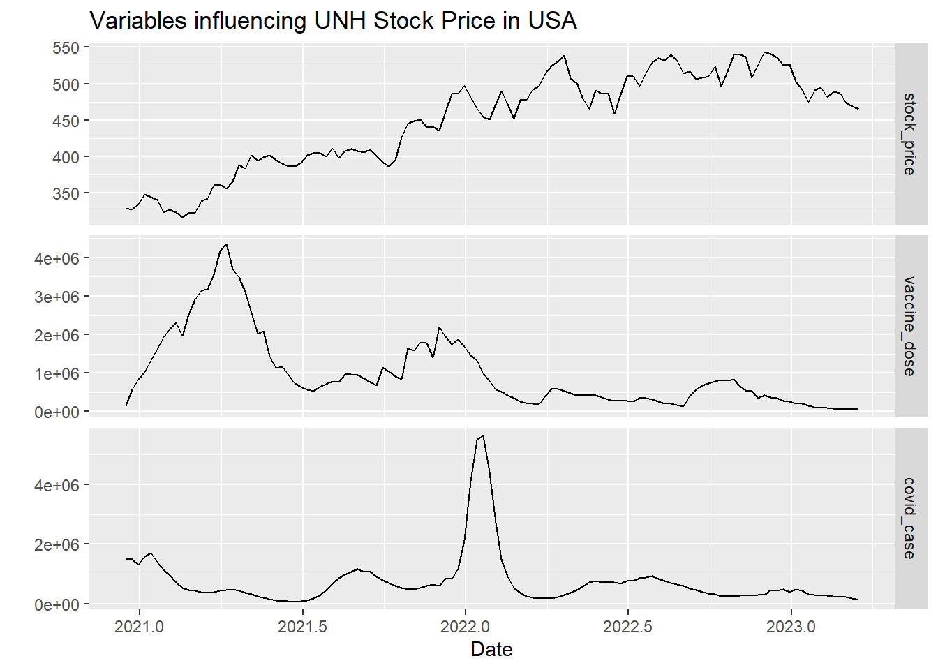

UNH stock price, Covid, Vaccine values

Step 3: Fitting the model using ’auto.arima()`

Here I’m using auto.arima() function to fit the ARIMAX model. Here we are trying to predict UNH stock price using COVID vaccine dose and COVID cases. All variables are time series and the exogenous variables in this case are vaccine_dose and covid_case.

Show the code

xreg <- cbind(Vac = df.ts[, "vaccine_dose"],
              Imp = df.ts[, "covid_case"])

fit <- auto.arima(df.ts[, "stock_price"], xreg = xreg)
summary(fit)

Series: df.ts[, "stock_price"] 
Regression with ARIMA(0,1,0) errors 

Coefficients:
        Vac    Imp
      0e+00  0e+00
s.e.  1e-04  1e-04

sigma^2 = 177.9:  log likelihood = -468.1
AIC=942.2   AICc=942.41   BIC=950.49

Training set error measures:
                   ME     RMSE      MAE      MPE     MAPE      MASE       ACF1
Training set 1.097616 13.16639 10.30662 0.233993 2.273228 0.1046469 0.04011524

Show the code

checkresiduals(fit)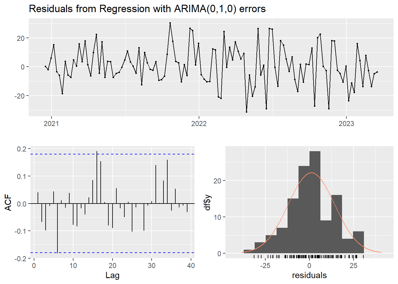

    Ljung-Box test

data:  Residuals from Regression with ARIMA(0,1,0) errors
Q* = 21.112, df = 24, p-value = 0.6321

Model df: 0.   Total lags used: 24

This is an ARIMA model. This is a Regression model with ARIMA(0,1,0) errors.

Step 4: Fitting the model manually

Here we will first have to fit the linear regression model predicting stock price using Covid cases and vaccine doses.

Then for the residuals, we will fit an ARIMA/SARIMA model.

Show the code

df$stock_price <- ts(df$stock_price,star=decimal_date(as.Date("2020-12-16",format = "%Y-%m-%d")),frequency = 52)
df$vaccine_dose <-ts(df$vaccine_dose,star=decimal_date(as.Date("2020-12-16",format = "%Y-%m-%d")),frequency = 52)
df$covid_case<-ts(df$covid_case,star=decimal_date(as.Date("2020-12-16",format = "%Y-%m-%d")),frequency = 52)

######### First fit the linear model#######
fit.reg <- lm(stock_price ~ vaccine_dose+covid_case, data=df)
summary(fit.reg)

Call:
lm(formula = stock_price ~ vaccine_dose + covid_case, data = df)

Residuals:
    Min      1Q  Median      3Q     Max 
-154.24  -42.59    8.62   42.91   82.36 

Coefficients:
               Estimate Std. Error t value Pr(>|t|)    
(Intercept)   4.954e+02  7.932e+00  62.461  < 2e-16 ***
vaccine_dose -4.341e-05  5.043e-06  -8.607 4.47e-14 ***
covid_case   -3.275e-06  5.345e-06  -0.613    0.541    
---
Signif. codes:  0 '***' 0.001 '**' 0.01 '*' 0.05 '.' 0.1 ' ' 1

Residual standard error: 52.02 on 115 degrees of freedom
Multiple R-squared:  0.3944,    Adjusted R-squared:  0.3839 
F-statistic: 37.45 on 2 and 115 DF,  p-value: 2.988e-13

Show the code

res.fit<-ts(residuals(fit.reg),star=decimal_date(as.Date("2020-12-16",format = "%Y-%m-%d")),frequency = 52)

########## Then look at the residuals ########
acf(res.fit)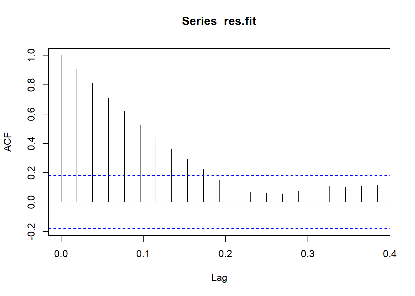

Show the code

Pacf(res.fit)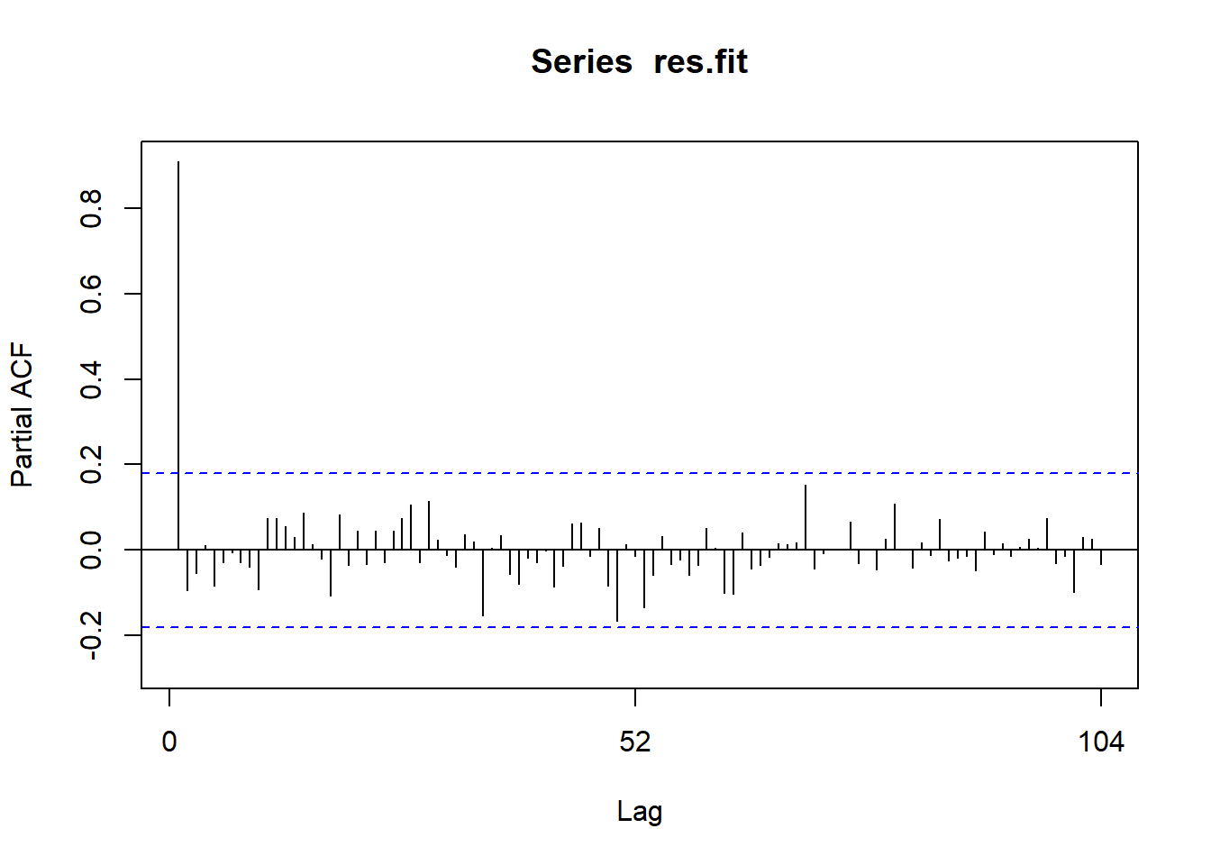

Show the code

res.fit %>% diff() %>% ggtsdisplay()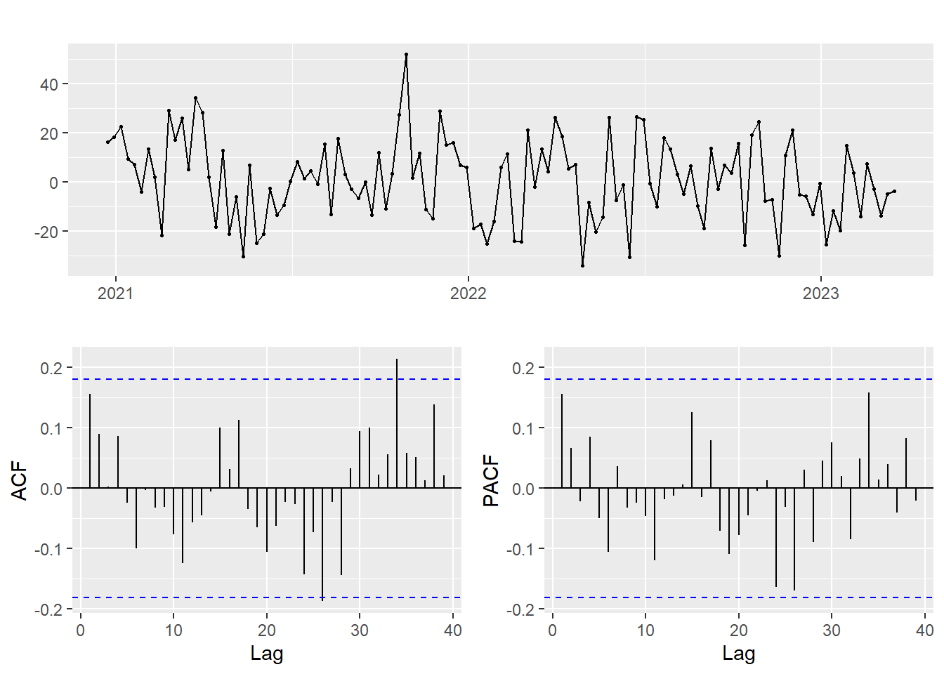

Show the code

res.fit %>% diff() %>% diff(52) %>% ggtsdisplay()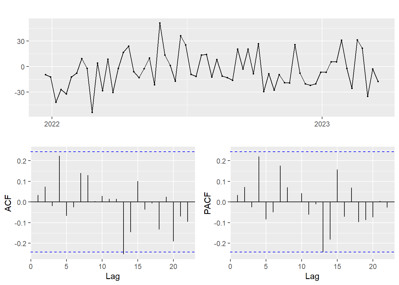

Finding the model parameters.

Show the code

d=1
i=1
temp= data.frame()
ls=matrix(rep(NA,6*23),nrow=23) # roughly nrow = 3x4x2


for (p in 1:3)# p=1,2,
{
  for(q in 1:3)# q=1,2,
  {
    for(d in 0:1)# 
    {
      
      if(p-1+d+q-1<=8)
      {
        
        model<- Arima(res.fit,order=c(p-1,d,q-1),include.drift=TRUE) 
        ls[i,]= c(p-1,d,q-1,model$aic,model$bic,model$aicc)
        i=i+1
        #print(i)
        
      }
      
    }
  }
}

temp= as.data.frame(ls)
names(temp)= c("p","d","q","AIC","BIC","AICc")

#temp
knitr::kable(temp)

p	d	q	AIC	BIC	AICc
0	0	0	1217.4187	1225.7307	1217.6292
0	1	0	993.5902	999.1146	993.6955
0	0	1	1117.7725	1128.8552	1118.1264
0	1	1	993.1256	1001.4121	993.3380
0	0	2	1058.3969	1072.2503	1058.9326
0	1	2	994.2046	1005.2533	994.5617
1	0	0	1005.4074	1016.4901	1005.7614
1	1	0	992.7214	1001.0079	992.9338
1	0	1	1003.8974	1017.7508	1004.4331
1	1	1	994.2405	1005.2892	994.5976
1	0	2	1003.9563	1020.5804	1004.7130
1	1	2	995.7980	1009.6089	996.3386
2	0	0	1002.8800	1016.7334	1003.4157
2	1	0	994.1790	1005.2277	994.5362
2	0	1	999.6163	1016.2404	1000.3730
2	1	1	995.8971	1009.7080	996.4376
2	0	2	1005.7699	1025.1647	1006.7881
2	1	2	995.6381	1012.2111	996.4017
NA	NA	NA	NA	NA	NA
NA	NA	NA	NA	NA	NA
NA	NA	NA	NA	NA	NA
NA	NA	NA	NA	NA	NA
NA	NA	NA	NA	NA	NA

Show the code

print('Minimum AIC')

[1] "Minimum AIC"

Show the code

temp[which.min(temp$AIC),] 

  p d q      AIC      BIC     AICc
8 1 1 0 992.7214 1001.008 992.9338

Show the code

print('Minimum BIC')

[1] "Minimum BIC"

Show the code

temp[which.min(temp$BIC),] 

  p d q      AIC      BIC     AICc
2 0 1 0 993.5902 999.1146 993.6955

Show the code

print('Minimum AICc')

[1] "Minimum AICc"

Show the code

temp[which.min(temp$AICc),] 

  p d q      AIC      BIC     AICc
8 1 1 0 992.7214 1001.008 992.9338

Show the code

set.seed(1234)

model_output12 <- capture.output(sarima(res.fit, 0,1,0))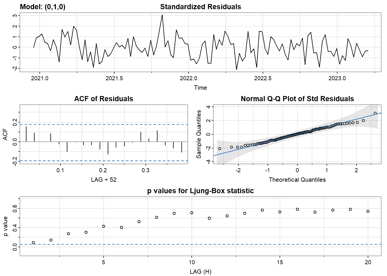 

Show the code

cat(model_output12[9:38], model_output12[length(model_output12)], sep = "\n")

$fit

Call:
arima(x = xdata, order = c(p, d, q), seasonal = list(order = c(P, D, Q), period = S), 
    xreg = constant, transform.pars = trans, fixed = fixed, optim.control = list(trace = trc, 
        REPORT = 1, reltol = tol))

Coefficients:
      constant
        1.0885
s.e.    1.5357

sigma^2 estimated as 275.9:  log likelihood = -494.8,  aic = 993.59

$degrees_of_freedom
[1] 116

$ttable
         Estimate     SE t.value p.value
constant   1.0885 1.5357  0.7088  0.4799

$AIC
[1] 8.492224

$AICc
[1] 8.492522

$BIC
[1] 8.539441

Show the code

set.seed(1234)

model_output13 <- capture.output(sarima(res.fit, 1,1,0))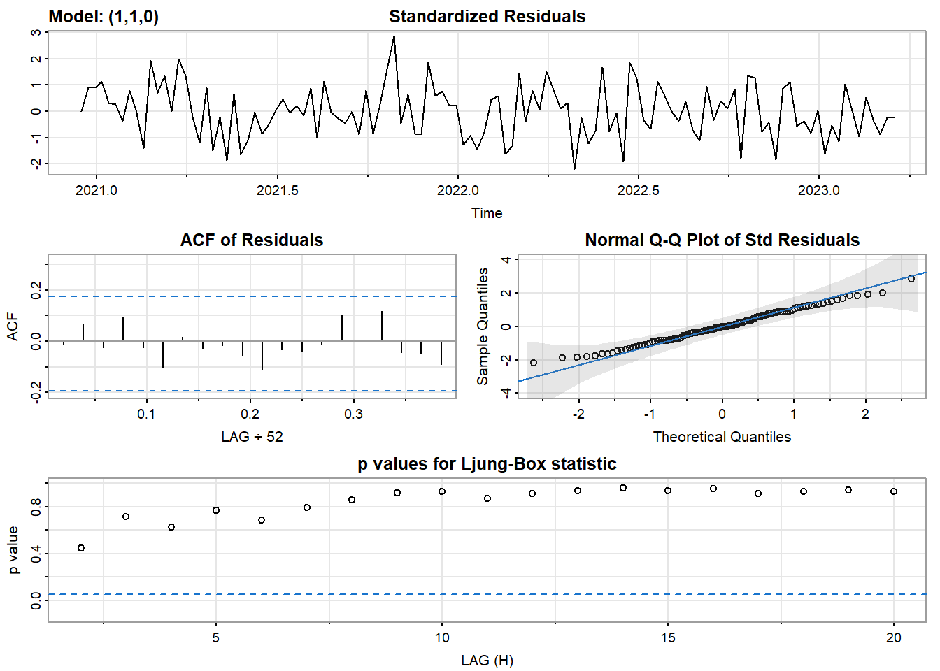 

Show the code

cat(model_output13[16:46], model_output13[length(model_output13)], sep = "\n")

$fit

Call:
arima(x = xdata, order = c(p, d, q), seasonal = list(order = c(P, D, Q), period = S), 
    xreg = constant, transform.pars = trans, fixed = fixed, optim.control = list(trace = trc, 
        REPORT = 1, reltol = tol))

Coefficients:
         ar1  constant
      0.1556    1.1047
s.e.  0.0913    1.7935

sigma^2 estimated as 269.2:  log likelihood = -493.36,  aic = 992.72

$degrees_of_freedom
[1] 115

$ttable
         Estimate     SE t.value p.value
ar1        0.1556 0.0913  1.7049  0.0909
constant   1.1047 1.7935  0.6160  0.5391

$AIC
[1] 8.484798

$AICc
[1] 8.485698

$BIC
[1] 8.555623

ARIMA(0,1,0) and ARIMA(1,1,0) both look okay.

Step 5: Using Cross Validation

Show the code

k <- 36 # minimum data length for fitting a model 
n <- length(res.fit)
n-k # rest of the observations

[1] 82

Show the code

i=1
err1 = c()
err2 = c()

rmse1 <- c()
rmse2 <- c()

for(i in 1:(n-k))
{
  xtrain <- res.fit[1:(k-1)+i] #observations from 1 to 75
  xtest <- res.fit[k+i] #76th observation as the test set
  
  fit <- Arima(xtrain, order=c(1,1,0),include.drift=FALSE, method="ML")
  fcast1 <- forecast(fit, h=1)
  
  fit2 <- Arima(xtrain, order=c(0,1,0),include.drift=FALSE, method="ML")
  fcast2 <- forecast(fit2, h=1)
  
  #capture error for each iteration
  # This is mean absolute error
  err1 = c(err1, abs(fcast1$mean-xtest)) 
  err2 = c(err2, abs(fcast2$mean-xtest))
  
  # This is mean squared error
  err3 = c(err1, (fcast1$mean-xtest)^2)
  err4 = c(err2, (fcast2$mean-xtest)^2)
  
  rmse1 <- c(rmse1, sqrt((fcast1$mean-xtest)^2))
  rmse2 <- c(rmse2, sqrt((fcast2$mean-xtest)^2))
  
}

(MAE1=mean(err1)) # This is mean absolute error

[1] 13.45554

Show the code

(MAE2=mean(err2)) #has slightly higher error

[1] 13.46804

Show the code

MSE1=mean(err1) #fit 1,1,0
MSE2=mean(err2)#fit 0,1,0

MSE1

[1] 13.45554

Show the code

MSE2

[1] 13.46804

Show the code

rmse_df <- data.frame(rmse1,rmse2)
rmse_df$x <- as.numeric(rownames(rmse_df))

plot(rmse_df$x, rmse_df$rmse1, type = 'l', col=2, xlab="horizon", ylab="RMSE")
lines(rmse_df$x, rmse_df$rmse2, type="l",col=3)
legend("topleft",legend=c("fit1","fit2"),col=2:4,lty=1)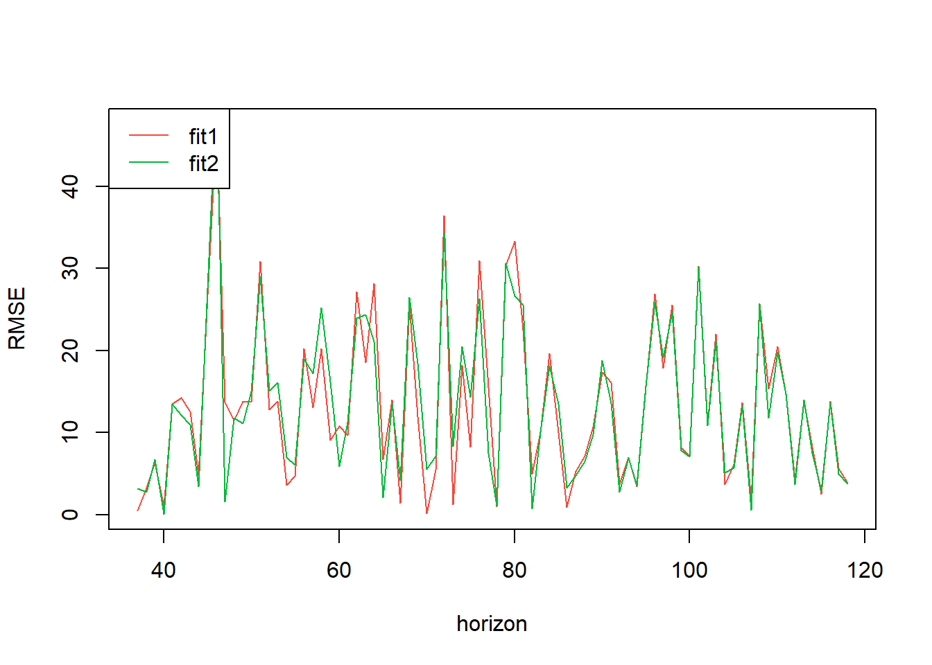

Step 6: forcasting

Show the code

vac_fit<-auto.arima(df$vaccine_dose) #fiting an ARIMA model to the vaccine_dose variable
summary(vac_fit)

Series: df$vaccine_dose 
ARIMA(1,1,1) 

Coefficients:
         ar1      ma1
      0.8341  -0.6298
s.e.  0.0916   0.1128

sigma^2 = 4.824e+10:  log likelihood = -1604.18
AIC=3214.36   AICc=3214.57   BIC=3222.65

Training set error measures:
                    ME     RMSE      MAE          MPE     MAPE      MASE
Training set -1592.486 216829.1 132002.8 0.0009291879 13.08388 0.1149613
                    ACF1
Training set -0.06829849

Show the code

fvac<-forecast(vac_fit)

covid_fit<-auto.arima(df$covid_case) #fiting an ARIMA model to the covid_case variable
summary(covid_fit)

Series: df$covid_case 
ARIMA(2,0,2) with non-zero mean 

Coefficients:
         ar1      ar2     ma1     ma2      mean
      1.3306  -0.5128  0.8165  0.4848  733469.2
s.e.  0.1153   0.1117  0.1363  0.1076  189902.4

sigma^2 = 2.904e+10:  log likelihood = -1588.94
AIC=3189.87   AICc=3190.63   BIC=3206.5

Training set error measures:
                    ME     RMSE      MAE       MPE     MAPE      MASE
Training set -424.0988 166757.6 99191.78 -6.959882 17.02194 0.1095754
                    ACF1
Training set -0.00122146

Show the code

fcov<-forecast(covid_fit)

fxreg <- cbind(Vac = fvac$mean,
              Cov = fcov$mean)

fcast <- forecast(fit, xreg=fxreg) #fimp$mean gives the forecasted values

Warning in forecast.forecast_ARIMA(fit, xreg = fxreg): xreg not required by this
model, ignoring the provided regressors

Show the code

autoplot(fcast) + xlab("Date") +
  ylab("Price")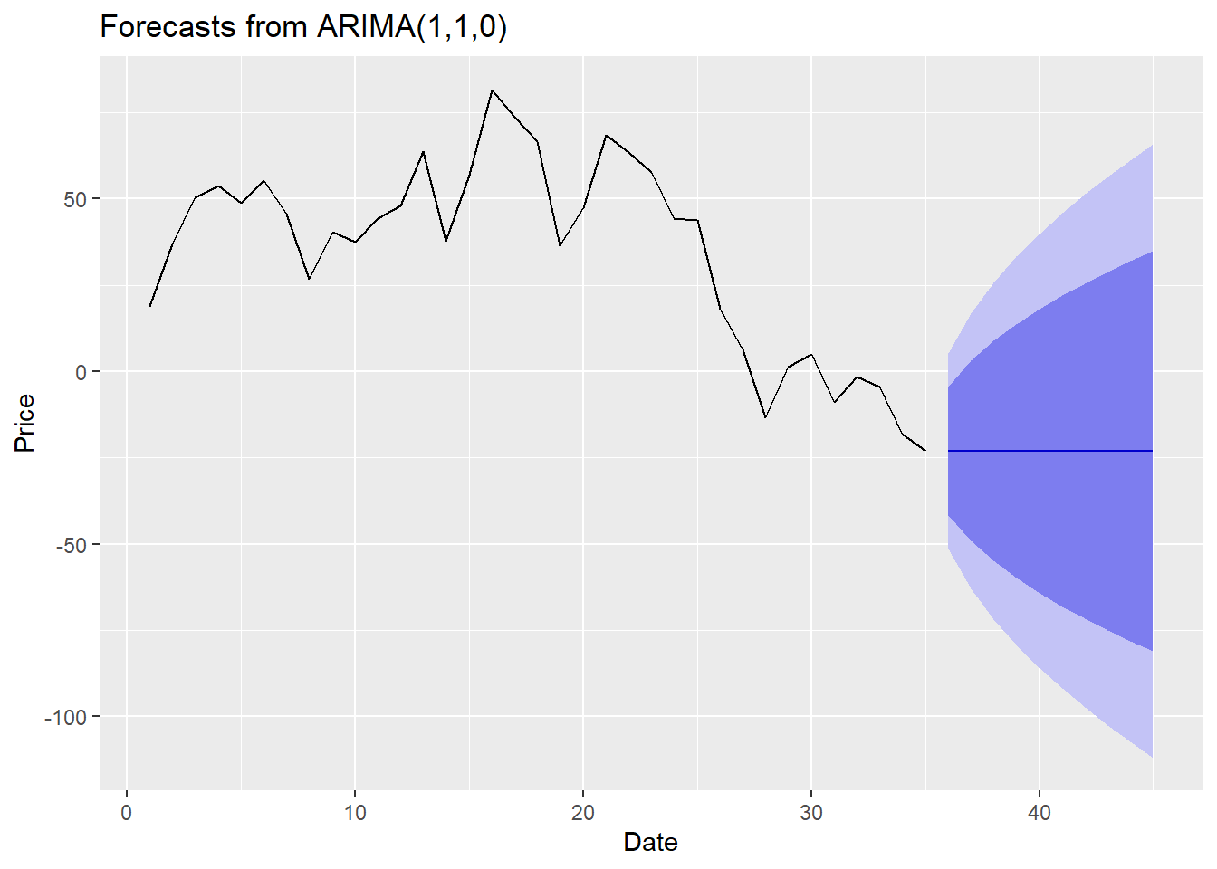

Discussion

Based on the result above, the number of daily COVID-19 vaccination number is not significant on predicting the UNH stock price, while the number of COVID-19 cases is. Though the number of COVID-19 vaccination number is not significant here, it does not mean that it does not affect healthcare stock price. While UNH is a healthcare company that is involved in health insurance, healthcare services, and technology solutions, it is not directly involved in COVID-19 vaccine development or production. Therefore, the number of COVID-19 vaccine doses administered may not have a direct impact on UNH’s operations or revenue.

VAR

VAR models (vector autoregressive models) are used for multivariate time series. The structure is that each variable is a linear function of past lags of itself and past lags of the other variables. A Vector autoregressive (VAR) model is useful when one is interested in predicting multiple time series variables using a single model.

The variables we are interested here are GDP and Unemployment rate in US. The overall health of the economy, as reflected by the GDP, can influence healthcare stock prices. A strong GDP generally indicates a healthy economy with higher levels of consumer spending, business investment, and economic growth. In such an environment, healthcare companies may experience increased demand for their products and services, which could positively impact their stock prices. Conversely, a weak GDP may signal an economic slowdown or recession, which could result in reduced demand for healthcare products and services, potentially leading to lower stock prices for healthcare companies. The unemployment rate, which reflects the percentage of the labor force that is unemployed, can also affect healthcare stock prices. A low unemployment rate is generally indicative of a strong labor market, with more people employed and potentially having access to employer-sponsored healthcare benefits. This may result in increased demand for healthcare services, positively impacting healthcare stock prices. On the other hand, a high unemployment rate may indicate a weak labor market, with more people losing their jobs and potentially losing access to healthcare benefits, leading to reduced demand for healthcare services and potentially lower stock prices for healthcare companies.

In this section, I’m fitting a VAR model to find multivariate relationship between the series UNH stock price, GDP, and Employment.

Step 1: Data Preparing

Show the code

getSymbols("UNH", from="1989-12-29", src="yahoo")

[1] "UNH"

Show the code

UNH_df <- as.data.frame(UNH)
UNH_df$Date <- rownames(UNH_df)
UNH_df <- UNH_df[c('Date','UNH.Adjusted')]
UNH_df <- UNH_df %>%
  mutate(Date = as.Date(Date)) %>%
  complete(Date = seq.Date(min(Date), max(Date), by="day"))

# fill missing values in stock 
UNH_df <- UNH_df %>% fill(UNH.Adjusted)
#UNH_df
new_dates <- seq(as.Date('1990-01-01'), as.Date('2022-10-01'),'quarter')
#new_dates
UNH_df <- UNH_df[which((UNH_df$Date) %in% new_dates),]

gdp <- read.csv('data/GDP59.CSV')
gdp$DATE <- as.Date(gdp$DATE)
gdp <- gdp[which((gdp$DATE) %in% new_dates),]

emp <- read.csv('data/Employment59.CSV')
emp$DATE <- as.Date(emp$DATE)
emp <- emp[which((emp$DATE) %in% new_dates),]

Show the code

dd <- data.frame(UNH_df,gdp,emp)
dd <- dd[,c(1,2,4,6)]
colnames(dd) <- c('DATE', 'stock_price','GDP','Employment')
knitr::kable(head(dd))

	DATE	stock_price	GDP	Employment
125	1990-01-01	0.308110	5872.701	109418.7
126	1990-04-01	0.247759	5960.028	109786.7
127	1990-07-01	0.438343	6015.116	109651.0
128	1990-10-01	0.435356	6004.733	109255.0
129	1991-01-01	0.591069	6035.178	108783.0
130	1991-04-01	0.985114	6126.862	108312.3

Step 2: Plotting the data

Show the code

dd.ts<-ts(dd,star=decimal_date(as.Date("1990-01-01",format = "%Y-%m-%d")),frequency = 4)

autoplot(dd.ts[,c(2:4)], facets=TRUE) +
  xlab("Year") + ylab("") +
  ggtitle("UNH Stock Price, GDP and Employment in USA")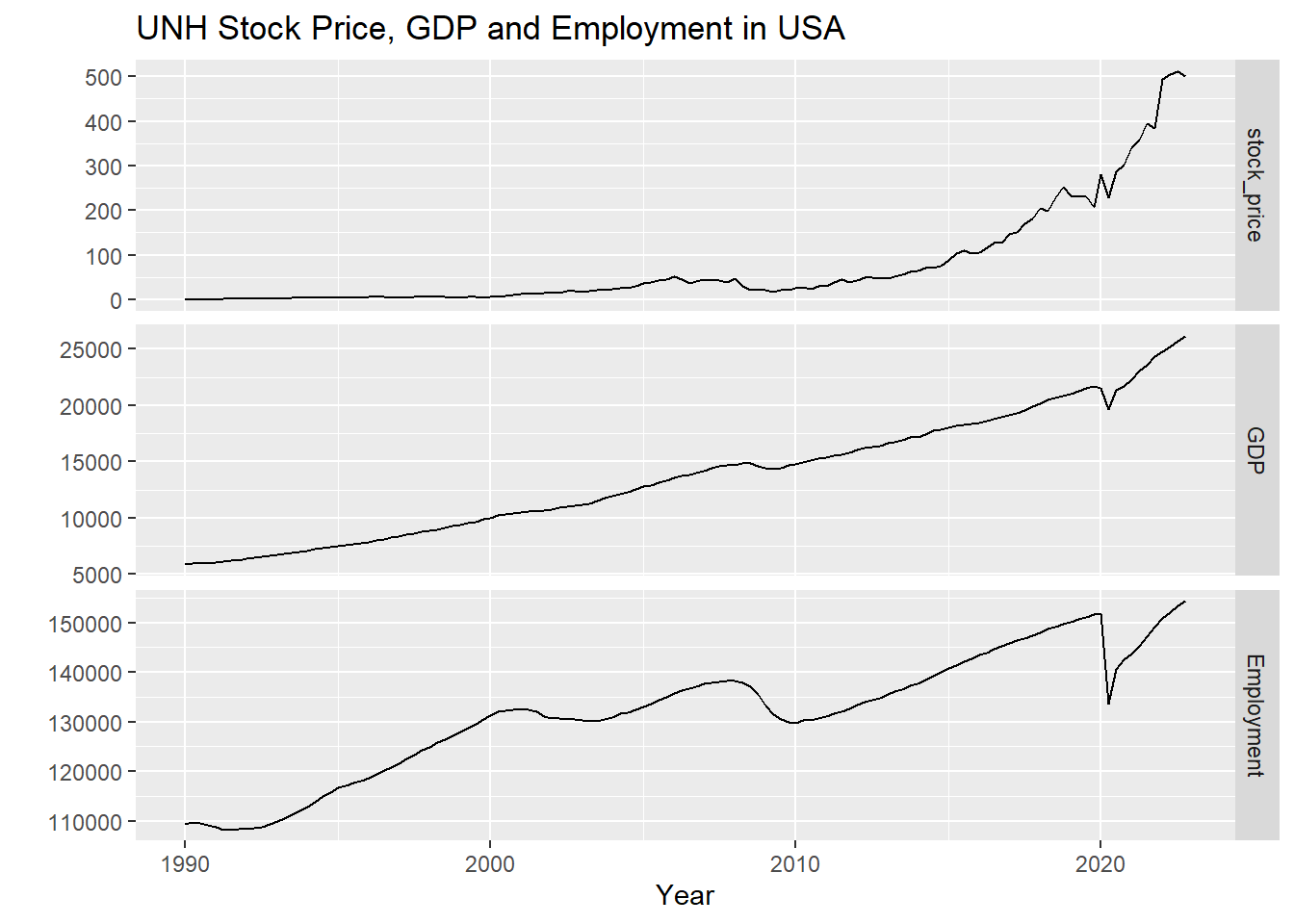

Step 3: Fitting a VAR model

Show the code

VARselect(dd[, c(2:4)], lag.max=10, type="both")

$selection
AIC(n)  HQ(n)  SC(n) FPE(n) 
    10      9      9      9 

$criteria
                  1            2            3            4            5
AIC(n) 2.941404e+01 2.865601e+01 2.849637e+01 2.814189e+01 2.812288e+01
HQ(n)  2.955407e+01 2.888005e+01 2.880444e+01 2.853398e+01 2.859898e+01
SC(n)  2.975880e+01 2.920762e+01 2.925484e+01 2.910721e+01 2.929506e+01
FPE(n) 5.948597e+12 2.788633e+12 2.379347e+12 1.671830e+12 1.644336e+12
                  6            7            8            9           10
AIC(n) 2.758294e+01 2.723307e+01 2.696700e+01 2.669062e+01 2.668670e+01
HQ(n)  2.814305e+01 2.787720e+01 2.769516e+01 2.750279e+01 2.758289e+01
SC(n)  2.896196e+01 2.881895e+01 2.875974e+01 2.869021e+01 2.889314e+01
FPE(n) 9.616264e+11 6.809549e+11 5.251270e+11 4.014819e+11 4.038690e+11

It’s clear that according to selection criteria p=10 and 9 are good.

I’m fitting several models with p=1(for simplicity), 5, and 9.=> VAR(1), VAR(5), VAR(9)

Show the code

summary(VAR(dd[, c(2:4)], p=1, type='both'))

VAR Estimation Results:
========================= 
Endogenous variables: stock_price, GDP, Employment 
Deterministic variables: both 
Sample size: 131 
Log Likelihood: -2461.36 
Roots of the characteristic polynomial:
1.028 0.9422  0.78
Call:
VAR(y = dd[, c(2:4)], p = 1, type = "both")


Estimation results for equation stock_price: 
============================================ 
stock_price = stock_price.l1 + GDP.l1 + Employment.l1 + const + trend 

                 Estimate Std. Error t value Pr(>|t|)    
stock_price.l1  1.0341243  0.0394781  26.195   <2e-16 ***
GDP.l1         -0.0005115  0.0039797  -0.129   0.8979    
Employment.l1  -0.0006163  0.0003038  -2.029   0.0446 *  
const          69.2145818 34.7475964   1.992   0.0485 *  
trend           0.3006699  0.4555344   0.660   0.5104    
---
Signif. codes:  0 '***' 0.001 '**' 0.01 '*' 0.05 '.' 0.1 ' ' 1


Residual standard error: 14.62 on 126 degrees of freedom
Multiple R-Squared: 0.9849, Adjusted R-squared: 0.9844 
F-statistic:  2057 on 4 and 126 DF,  p-value: < 2.2e-16 


Estimation results for equation GDP: 
==================================== 
GDP = stock_price.l1 + GDP.l1 + Employment.l1 + const + trend 

                 Estimate Std. Error t value Pr(>|t|)    
stock_price.l1    2.55503    0.64584   3.956 0.000126 ***
GDP.l1            0.79020    0.06511  12.137  < 2e-16 ***
Employment.l1    -0.01069    0.00497  -2.151 0.033349 *  
const          2355.16290  568.45522   4.143 6.24e-05 ***
trend            27.89290    7.45234   3.743 0.000275 ***
---
Signif. codes:  0 '***' 0.001 '**' 0.01 '*' 0.05 '.' 0.1 ' ' 1


Residual standard error: 239.2 on 126 degrees of freedom
Multiple R-Squared: 0.998,  Adjusted R-squared: 0.998 
F-statistic: 1.607e+04 on 4 and 126 DF,  p-value: < 2.2e-16 


Estimation results for equation Employment: 
=========================================== 
Employment = stock_price.l1 + GDP.l1 + Employment.l1 + const + trend 

                 Estimate Std. Error t value Pr(>|t|)    
stock_price.l1  6.183e+00  4.862e+00   1.272  0.20584    
GDP.l1         -5.610e-01  4.901e-01  -1.145  0.25458    
Employment.l1   9.253e-01  3.741e-02  24.733  < 2e-16 ***
const           1.161e+04  4.279e+03   2.712  0.00762 ** 
trend           8.544e+01  5.610e+01   1.523  0.13028    
---
Signif. codes:  0 '***' 0.001 '**' 0.01 '*' 0.05 '.' 0.1 ' ' 1


Residual standard error: 1801 on 126 degrees of freedom
Multiple R-Squared: 0.9786, Adjusted R-squared: 0.9779 
F-statistic:  1441 on 4 and 126 DF,  p-value: < 2.2e-16 



Covariance matrix of residuals:
            stock_price    GDP Employment
stock_price       213.8   1386      12148
GDP              1385.8  57224     396720
Employment      12147.6 396720    3242998

Correlation matrix of residuals:
            stock_price    GDP Employment
stock_price      1.0000 0.3962     0.4613
GDP              0.3962 1.0000     0.9209
Employment       0.4613 0.9209     1.0000

Show the code

summary(VAR(dd[, c(2:4)], p=5, type='both'))

VAR Estimation Results:
========================= 
Endogenous variables: stock_price, GDP, Employment 
Deterministic variables: both 
Sample size: 127 
Log Likelihood: -2267.863 
Roots of the characteristic polynomial:
1.054 0.9435 0.9435 0.8781 0.8781 0.7952 0.7952 0.7806 0.7806 0.7709 0.7709 0.6959 0.4107 0.4107 0.3355
Call:
VAR(y = dd[, c(2:4)], p = 5, type = "both")


Estimation results for equation stock_price: 
============================================ 
stock_price = stock_price.l1 + GDP.l1 + Employment.l1 + stock_price.l2 + GDP.l2 + Employment.l2 + stock_price.l3 + GDP.l3 + Employment.l3 + stock_price.l4 + GDP.l4 + Employment.l4 + stock_price.l5 + GDP.l5 + Employment.l5 + const + trend 

                 Estimate Std. Error t value Pr(>|t|)    
stock_price.l1  5.454e-01  1.048e-01   5.204 9.13e-07 ***
GDP.l1          6.007e-02  1.789e-02   3.358  0.00108 ** 
Employment.l1  -7.709e-03  2.385e-03  -3.232  0.00162 ** 
stock_price.l2  2.323e-01  1.468e-01   1.583  0.11639    
GDP.l2         -6.188e-02  2.695e-02  -2.297  0.02353 *  
Employment.l2   8.708e-03  4.117e-03   2.115  0.03668 *  
stock_price.l3 -6.701e-02  1.636e-01  -0.410  0.68293    
GDP.l3          1.256e-02  2.614e-02   0.480  0.63198    
Employment.l3  -3.778e-03  4.122e-03  -0.917  0.36136    
stock_price.l4  2.159e-01  1.796e-01   1.202  0.23192    
GDP.l4         -1.114e-02  2.275e-02  -0.490  0.62525    
Employment.l4   2.759e-03  3.733e-03   0.739  0.46146    
stock_price.l5  2.480e-01  1.956e-01   1.268  0.20751    
GDP.l5         -1.060e-02  1.379e-02  -0.769  0.44375    
Employment.l5  -6.394e-04  2.197e-03  -0.291  0.77155    
const           1.189e+02  3.723e+01   3.194  0.00183 ** 
trend           1.493e+00  5.610e-01   2.661  0.00897 ** 
---
Signif. codes:  0 '***' 0.001 '**' 0.01 '*' 0.05 '.' 0.1 ' ' 1


Residual standard error: 12.06 on 110 degrees of freedom
Multiple R-Squared: 0.9909, Adjusted R-squared: 0.9896 
F-statistic: 750.5 on 16 and 110 DF,  p-value: < 2.2e-16 


Estimation results for equation GDP: 
==================================== 
GDP = stock_price.l1 + GDP.l1 + Employment.l1 + stock_price.l2 + GDP.l2 + Employment.l2 + stock_price.l3 + GDP.l3 + Employment.l3 + stock_price.l4 + GDP.l4 + Employment.l4 + stock_price.l5 + GDP.l5 + Employment.l5 + const + trend 

                 Estimate Std. Error t value Pr(>|t|)    
stock_price.l1   -1.30445    1.54245  -0.846 0.399555    
GDP.l1            1.92765    0.26327   7.322 4.28e-11 ***
Employment.l1    -0.18525    0.03510  -5.277 6.65e-07 ***
stock_price.l2    7.85075    2.15990   3.635 0.000425 ***
GDP.l2           -0.49800    0.39656  -1.256 0.211852    
Employment.l2     0.14315    0.06059   2.363 0.019907 *  
stock_price.l3    1.97665    2.40806   0.821 0.413510    
GDP.l3           -0.68441    0.38474  -1.779 0.078023 .  
Employment.l3     0.07846    0.06066   1.293 0.198571    
stock_price.l4   -3.50097    2.64351  -1.324 0.188127    
GDP.l4           -0.53338    0.33481  -1.593 0.114012    
Employment.l4     0.03338    0.05493   0.608 0.544643    
stock_price.l5   -4.52830    2.87918  -1.573 0.118643    
GDP.l5            0.62554    0.20300   3.081 0.002603 ** 
Employment.l5    -0.07633    0.03233  -2.361 0.019978 *  
const          1593.63764  547.91857   2.909 0.004394 ** 
trend            21.22796    8.25642   2.571 0.011473 *  
---
Signif. codes:  0 '***' 0.001 '**' 0.01 '*' 0.05 '.' 0.1 ' ' 1


Residual standard error: 177.5 on 110 degrees of freedom
Multiple R-Squared: 0.999,  Adjusted R-squared: 0.9988 
F-statistic:  6815 on 16 and 110 DF,  p-value: < 2.2e-16 


Estimation results for equation Employment: 
=========================================== 
Employment = stock_price.l1 + GDP.l1 + Employment.l1 + stock_price.l2 + GDP.l2 + Employment.l2 + stock_price.l3 + GDP.l3 + Employment.l3 + stock_price.l4 + GDP.l4 + Employment.l4 + stock_price.l5 + GDP.l5 + Employment.l5 + const + trend 

                 Estimate Std. Error t value Pr(>|t|)    
stock_price.l1 -3.786e+01  1.190e+01  -3.182  0.00190 ** 
GDP.l1          6.787e+00  2.030e+00   3.343  0.00113 ** 
Employment.l1  -1.385e-02  2.707e-01  -0.051  0.95928    
stock_price.l2  7.770e+01  1.666e+01   4.664 8.77e-06 ***
GDP.l2         -2.705e+00  3.058e+00  -0.885  0.37831    
Employment.l2   6.207e-01  4.673e-01   1.328  0.18686    
stock_price.l3  4.014e+00  1.857e+01   0.216  0.82927    
GDP.l3         -8.103e+00  2.967e+00  -2.731  0.00736 ** 
Employment.l3   1.098e+00  4.678e-01   2.346  0.02075 *  
stock_price.l4 -1.641e+01  2.039e+01  -0.805  0.42269    
GDP.l4         -1.499e+00  2.582e+00  -0.581  0.56270    
Employment.l4  -1.900e-01  4.237e-01  -0.448  0.65470    
stock_price.l5 -2.700e+01  2.221e+01  -1.216  0.22657    
GDP.l5          4.674e+00  1.566e+00   2.985  0.00349 ** 
Employment.l5  -5.865e-01  2.493e-01  -2.352  0.02044 *  
const           1.222e+04  4.226e+03   2.891  0.00462 ** 
trend           1.203e+02  6.368e+01   1.890  0.06146 .  
---
Signif. codes:  0 '***' 0.001 '**' 0.01 '*' 0.05 '.' 0.1 ' ' 1


Residual standard error: 1369 on 110 degrees of freedom
Multiple R-Squared: 0.9879, Adjusted R-squared: 0.9861 
F-statistic: 560.4 on 16 and 110 DF,  p-value: < 2.2e-16 



Covariance matrix of residuals:
            stock_price      GDP Employment
stock_price       145.5    455.4       5503
GDP               455.4  31506.6     225145
Employment       5503.3 225144.8    1874014

Correlation matrix of residuals:
            stock_price    GDP Employment
stock_price      1.0000 0.2127     0.3333
GDP              0.2127 1.0000     0.9266
Employment       0.3333 0.9266     1.0000

Show the code

summary(VAR(dd[, c(2:4)], p=9, type='both'))

VAR Estimation Results:
========================= 
Endogenous variables: stock_price, GDP, Employment 
Deterministic variables: both 
Sample size: 123 
Log Likelihood: -2076.371 
Roots of the characteristic polynomial:
1.058 1.051 1.018 1.018 1.012 1.012 1.012 1.012 1.005 1.005 1.003 1.003 0.9793 0.9793 0.9726 0.9726 0.8256 0.8256 0.8098 0.8098 0.7926 0.7926 0.6662 0.6662 0.4868 0.4868 0.0237
Call:
VAR(y = dd[, c(2:4)], p = 9, type = "both")


Estimation results for equation stock_price: 
============================================ 
stock_price = stock_price.l1 + GDP.l1 + Employment.l1 + stock_price.l2 + GDP.l2 + Employment.l2 + stock_price.l3 + GDP.l3 + Employment.l3 + stock_price.l4 + GDP.l4 + Employment.l4 + stock_price.l5 + GDP.l5 + Employment.l5 + stock_price.l6 + GDP.l6 + Employment.l6 + stock_price.l7 + GDP.l7 + Employment.l7 + stock_price.l8 + GDP.l8 + Employment.l8 + stock_price.l9 + GDP.l9 + Employment.l9 + const + trend 

                 Estimate Std. Error t value Pr(>|t|)    
stock_price.l1  0.6177986  0.1140057   5.419 4.61e-07 ***
GDP.l1          0.0415175  0.0139527   2.976 0.003717 ** 
Employment.l1  -0.0069645  0.0020733  -3.359 0.001131 ** 
stock_price.l2  0.3603716  0.1652332   2.181 0.031680 *  
GDP.l2         -0.0157162  0.0211664  -0.743 0.459633    
Employment.l2   0.0048987  0.0033424   1.466 0.146093    
stock_price.l3  0.0177119  0.1607489   0.110 0.912499    
GDP.l3         -0.0009781  0.0212811  -0.046 0.963439    
Employment.l3  -0.0018913  0.0034992  -0.540 0.590135    
stock_price.l4 -0.1568989  0.1711382  -0.917 0.361596    
GDP.l4         -0.0352143  0.0218848  -1.609 0.110953    
Employment.l4   0.0072039  0.0035652   2.021 0.046168 *  
stock_price.l5  0.3383735  0.2044761   1.655 0.101294    
GDP.l5         -0.0156536  0.0222246  -0.704 0.482964    
Employment.l5   0.0016545  0.0036673   0.451 0.652934    
stock_price.l6  0.1416245  0.2112799   0.670 0.504299    
GDP.l6         -0.0184066  0.0221573  -0.831 0.408236    
Employment.l6  -0.0012687  0.0036506  -0.348 0.728965    
stock_price.l7 -0.9691876  0.2444899  -3.964 0.000144 ***
GDP.l7          0.0190303  0.0219980   0.865 0.389190    
Employment.l7  -0.0017353  0.0035712  -0.486 0.628163    
stock_price.l8  1.0643895  0.2599676   4.094 8.96e-05 ***
GDP.l8          0.0123808  0.0212167   0.584 0.560927    
Employment.l8  -0.0058935  0.0033845  -1.741 0.084893 .  
stock_price.l9 -0.2681893  0.2116088  -1.267 0.208149    
GDP.l9          0.0063637  0.0130395   0.488 0.626663    
Employment.l9   0.0035409  0.0021429   1.652 0.101786    
const          79.8647702 39.9369777   2.000 0.048411 *  
trend           0.9524397  0.5617195   1.696 0.093276 .  
---
Signif. codes:  0 '***' 0.001 '**' 0.01 '*' 0.05 '.' 0.1 ' ' 1


Residual standard error: 8.687 on 94 degrees of freedom
Multiple R-Squared: 0.9959, Adjusted R-squared: 0.9947 
F-statistic:   819 on 28 and 94 DF,  p-value: < 2.2e-16 


Estimation results for equation GDP: 
==================================== 
GDP = stock_price.l1 + GDP.l1 + Employment.l1 + stock_price.l2 + GDP.l2 + Employment.l2 + stock_price.l3 + GDP.l3 + Employment.l3 + stock_price.l4 + GDP.l4 + Employment.l4 + stock_price.l5 + GDP.l5 + Employment.l5 + stock_price.l6 + GDP.l6 + Employment.l6 + stock_price.l7 + GDP.l7 + Employment.l7 + stock_price.l8 + GDP.l8 + Employment.l8 + stock_price.l9 + GDP.l9 + Employment.l9 + const + trend 

                 Estimate Std. Error t value Pr(>|t|)    
stock_price.l1 -5.605e+00  1.777e+00  -3.154  0.00217 ** 
GDP.l1          1.818e+00  2.175e-01   8.360 5.58e-13 ***
Employment.l1  -1.497e-01  3.232e-02  -4.631 1.17e-05 ***
stock_price.l2  1.352e+01  2.576e+00   5.250 9.43e-07 ***
GDP.l2         -7.098e-01  3.300e-01  -2.151  0.03403 *  
Employment.l2   1.262e-01  5.211e-02   2.422  0.01734 *  
stock_price.l3 -1.116e+00  2.506e+00  -0.445  0.65722    
GDP.l3         -2.534e-01  3.318e-01  -0.764  0.44683    
Employment.l3   3.585e-02  5.455e-02   0.657  0.51262    
stock_price.l4  1.673e+00  2.668e+00   0.627  0.53208    
GDP.l4         -8.506e-02  3.412e-01  -0.249  0.80365    
Employment.l4   1.384e-02  5.558e-02   0.249  0.80384    
stock_price.l5 -7.495e-01  3.188e+00  -0.235  0.81462    
GDP.l5          1.171e-01  3.465e-01   0.338  0.73604    
Employment.l5  -2.497e-02  5.717e-02  -0.437  0.66327    
stock_price.l6 -1.389e+01  3.294e+00  -4.216 5.71e-05 ***
GDP.l6          2.705e-02  3.454e-01   0.078  0.93775    
Employment.l6  -9.452e-03  5.691e-02  -0.166  0.86846    
stock_price.l7 -1.613e+00  3.812e+00  -0.423  0.67319    
GDP.l7         -2.916e-01  3.429e-01  -0.850  0.39727    
Employment.l7   7.971e-02  5.567e-02   1.432  0.15551    
stock_price.l8  7.701e+00  4.053e+00   1.900  0.06049 .  
GDP.l8          9.947e-02  3.308e-01   0.301  0.76428    
Employment.l8  -1.132e-01  5.276e-02  -2.144  0.03457 *  
stock_price.l9  1.073e+00  3.299e+00   0.325  0.74571    
GDP.l9          1.156e-01  2.033e-01   0.569  0.57100    
Employment.l9   3.477e-02  3.341e-02   1.041  0.30064    
const           1.603e+03  6.226e+02   2.575  0.01159 *  
trend           2.134e+01  8.757e+00   2.437  0.01669 *  
---
Signif. codes:  0 '***' 0.001 '**' 0.01 '*' 0.05 '.' 0.1 ' ' 1


Residual standard error: 135.4 on 94 degrees of freedom
Multiple R-Squared: 0.9995, Adjusted R-squared: 0.9993 
F-statistic:  6211 on 28 and 94 DF,  p-value: < 2.2e-16 


Estimation results for equation Employment: 
=========================================== 
Employment = stock_price.l1 + GDP.l1 + Employment.l1 + stock_price.l2 + GDP.l2 + Employment.l2 + stock_price.l3 + GDP.l3 + Employment.l3 + stock_price.l4 + GDP.l4 + Employment.l4 + stock_price.l5 + GDP.l5 + Employment.l5 + stock_price.l6 + GDP.l6 + Employment.l6 + stock_price.l7 + GDP.l7 + Employment.l7 + stock_price.l8 + GDP.l8 + Employment.l8 + stock_price.l9 + GDP.l9 + Employment.l9 + const + trend 

                 Estimate Std. Error t value Pr(>|t|)    
stock_price.l1 -6.801e+01  1.216e+01  -5.595 2.17e-07 ***
GDP.l1          6.439e+00  1.488e+00   4.328 3.75e-05 ***
Employment.l1   1.372e-01  2.211e-01   0.621  0.53643    
stock_price.l2  1.137e+02  1.762e+01   6.453 4.74e-09 ***
GDP.l2         -4.116e+00  2.257e+00  -1.824  0.07136 .  
Employment.l2   5.335e-01  3.564e-01   1.497  0.13778    
stock_price.l3 -4.159e+00  1.714e+01  -0.243  0.80882    
GDP.l3         -3.838e+00  2.269e+00  -1.691  0.09408 .  
Employment.l3   5.003e-01  3.731e-01   1.341  0.18318    
stock_price.l4  1.066e+01  1.825e+01   0.584  0.56038    
GDP.l4         -6.501e-02  2.334e+00  -0.028  0.97783    
Employment.l4   1.168e-01  3.802e-01   0.307  0.75925    
stock_price.l5  2.259e+01  2.180e+01   1.036  0.30277    
GDP.l5          8.889e-01  2.370e+00   0.375  0.70845    
Employment.l5  -2.821e-01  3.911e-01  -0.721  0.47245    
stock_price.l6 -1.130e+02  2.253e+01  -5.017 2.48e-06 ***
GDP.l6         -1.567e+00  2.363e+00  -0.663  0.50891    
Employment.l6   2.161e-01  3.893e-01   0.555  0.58019    
stock_price.l7 -2.070e+01  2.607e+01  -0.794  0.42930    
GDP.l7         -1.096e+00  2.346e+00  -0.467  0.64133    
Employment.l7   4.753e-01  3.808e-01   1.248  0.21512    
stock_price.l8  8.864e+01  2.772e+01   3.198  0.00189 ** 
GDP.l8          1.933e+00  2.262e+00   0.854  0.39515    
Employment.l8  -1.204e+00  3.609e-01  -3.336  0.00122 ** 
stock_price.l9 -3.272e+01  2.256e+01  -1.450  0.15042    
GDP.l9          8.076e-01  1.390e+00   0.581  0.56273    
Employment.l9   4.222e-01  2.285e-01   1.848  0.06777 .  
const           1.262e+04  4.259e+03   2.963  0.00386 ** 
trend           9.703e+01  5.990e+01   1.620  0.10859    
---
Signif. codes:  0 '***' 0.001 '**' 0.01 '*' 0.05 '.' 0.1 ' ' 1


Residual standard error: 926.4 on 94 degrees of freedom
Multiple R-Squared: 0.9945, Adjusted R-squared: 0.9928 
F-statistic: 603.2 on 28 and 94 DF,  p-value: < 2.2e-16 



Covariance matrix of residuals:
            stock_price      GDP Employment
stock_price       75.47    290.5       2750
GDP              290.52  18342.3     112144
Employment      2749.66 112143.8     858125

Correlation matrix of residuals:
            stock_price    GDP Employment
stock_price      1.0000 0.2469     0.3417
GDP              0.2469 1.0000     0.8939
Employment       0.3417 0.8939     1.0000

Step 4: Using Cross Validation

Show the code

n=length(dd$stock_price)
k=39

#n-k=92; 92/4=23;

rmse1 <- matrix(NA, 96,3)
rmse2 <- matrix(NA, 96,3)
rmse3 <- matrix(NA,23,4)
year<-c()

# Convert data frame to time series object
ts_obj <- ts(dd[, c(2:4)], star=decimal_date(as.Date("1990-01-01",format = "%Y-%m-%d")),frequency = 4)

st <- tsp(ts_obj )[1]+(k-1)/4 


for(i in 1:23)
{
  
  xtrain <- window(ts_obj, end=st + i-1)
  xtest <- window(ts_obj, start=st + (i-1) + 1/4, end=st + i)
  
  
  fit <- VAR(ts_obj, p=5, type='both')
  fcast <- predict(fit, n.ahead = 4)
  
  fgdp<-fcast$fcst$GDP
  femp<-fcast$fcst$Employment
  fsp<-fcast$fcst$stock_price
  ff<-data.frame(fsp[,1],fgdp[,1],femp[,1])
  
  year<-st + (i-1) + 1/4
  
  ff<-ts(ff,start=c(year,1),frequency = 4)
  
  a = 4*i-3
  b= 4*i
  rmse1[c(a:b),]  <-sqrt((ff-xtest)^2)
  
  fit2 <- VAR(ts_obj, p=9, type='both')
  fcast2 <- predict(fit2, n.ahead = 4)
  
  fgdp<-fcast2$fcst$GDP
  femp<-fcast2$fcst$Employment
  fsp<-fcast2$fcst$stock_price
  ff2<-data.frame(fsp[,1],fgdp[,1],femp[,1])
  
  year<-st + (i-1) + 1/4
  
  ff2<-ts(ff2,start=c(year,1),frequency = 4)
  
  a = 4*i-3
  b= 4*i
  rmse2[c(a:b),]  <-sqrt((ff2-xtest)^2)
}

yr = rep(c(1999:2022),each =4)
qr = rep(paste0("Q",1:4),24)

rmse1 = data.frame(yr,qr,rmse1)
names(rmse1) =c("Year", "Quater","Stock_Price","GDP","Employment")
rmse2 = data.frame(yr,qr,rmse2)
names(rmse2) =c("Year", "Quater","Stock_Price","GDP","Employment")

ggplot() + 
  geom_line(data = rmse1, aes(x = Year, y = Stock_Price),color = "blue") +
  geom_line(data = rmse2, aes(x = Year, y = Stock_Price),color = "red") +
  labs(
    title = "CV RMSE for Stock_Price",
    x = "Date",
    y = "RMSE",
    guides(colour=guide_legend(title="Fit")))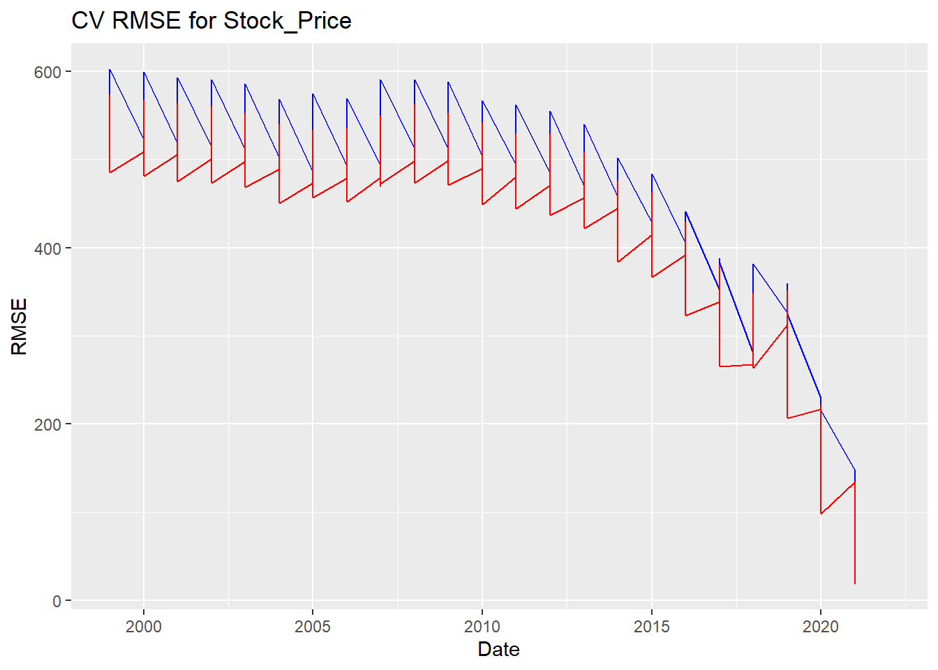

Show the code

ggplot() + 
  geom_line(data = rmse1, aes(x = Year, y = GDP),color = "blue") +
  geom_line(data = rmse2, aes(x = Year, y = GDP),color = "red") +
  labs(
    title = "CV RMSE for GDP",
    x = "Date",
    y = "RMSE",
    guides(colour=guide_legend(title="Fit")))

Warning: Removed 4 rows containing missing values (`geom_line()`).
Removed 4 rows containing missing values (`geom_line()`).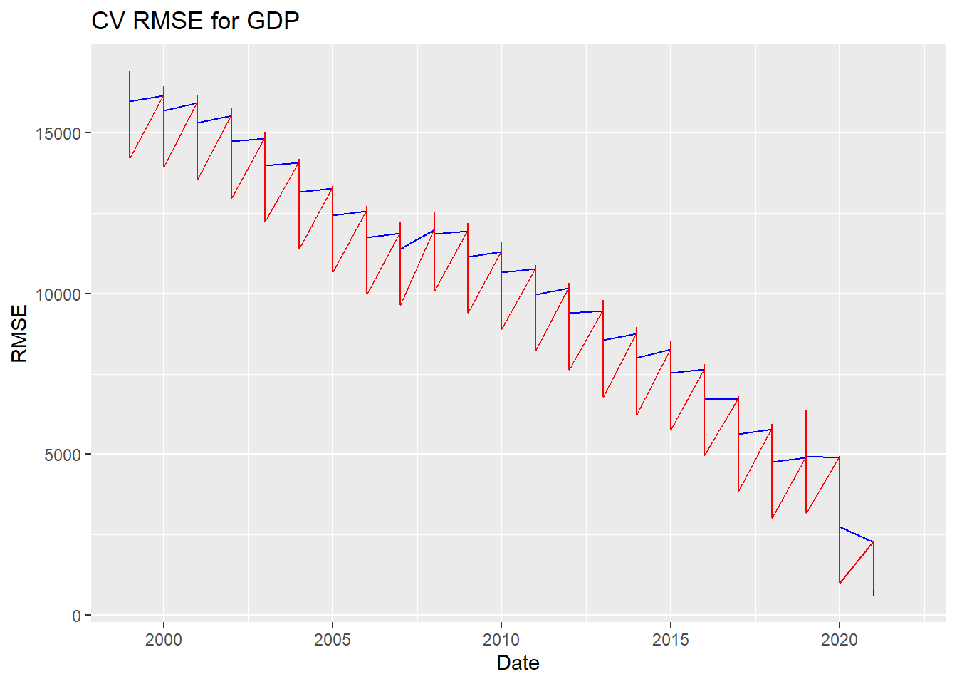

Show the code

ggplot() + 
  geom_line(data = rmse1, aes(x = Year, y = Employment),color = "blue") +
  geom_line(data = rmse2, aes(x = Year, y = Employment),color = "red") +
  labs(
    title = "CV RMSE for Employment",
    x = "Date",
    y = "RMSE",
    guides(colour=guide_legend(title="Fit")))

Warning: Removed 4 rows containing missing values (`geom_line()`).
Removed 4 rows containing missing values (`geom_line()`).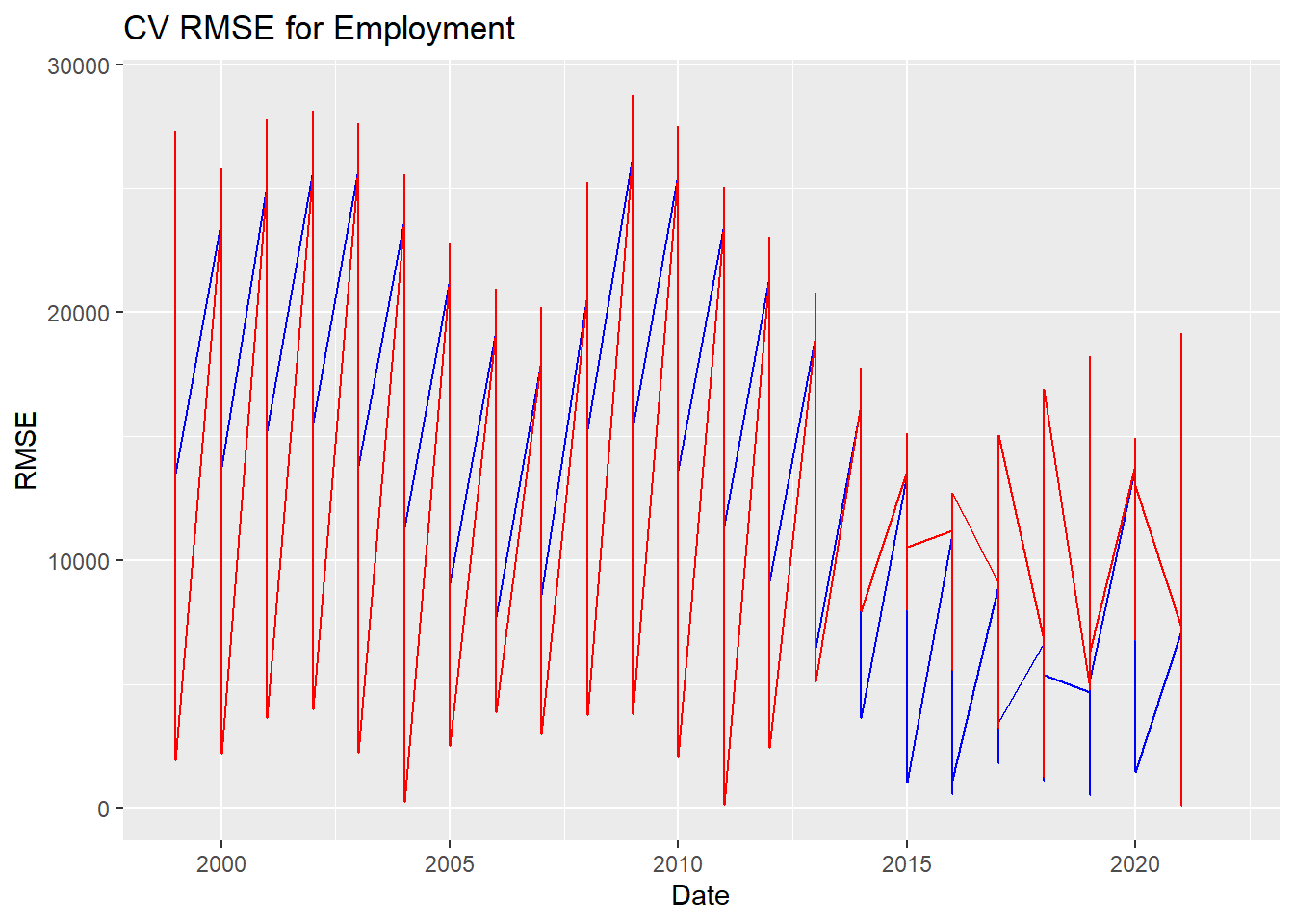

fit 1 is better

Step 5: Forecast

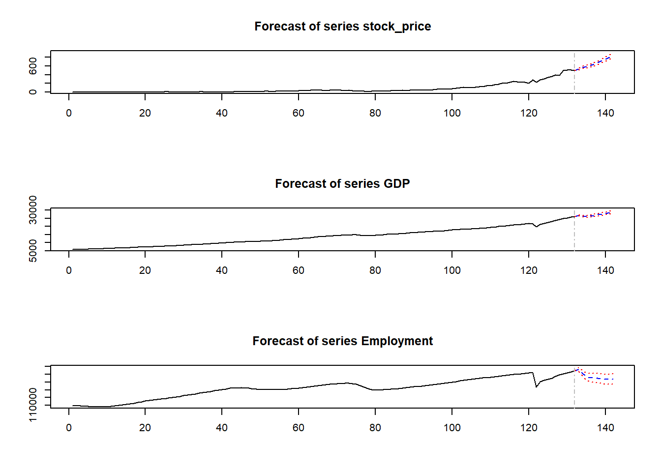
Show the code

forecasts <- predict(VAR(dd[, c(2:4)], p=5, type='both'))

# visualize the iterated forecasts
plot(forecasts)