Financial Time Series Models: CVS Example
Volatility is a statistical measure of the dispersion of returns for a given security or market index. In most cases, the higher the volatility, the riskier the security. It is often measured as either the standard deviation or variance between returns from the same security or market index.
At this section, I am going to fit financial time series models on CVS stock price.
Show the code
getSymbols("CVS", from="2010-1-1", src="yahoo")
CVS_df <- as.data.frame(CVS)
CVS_df$Date <- rownames(CVS_df)
CVS_df <- CVS_df[c('Date','CVS.Adjusted')]
CVS_df <- CVS_df %>%
  mutate(Date = as.Date(Date)) %>%
  complete(Date = seq.Date(min(Date), max(Date), by="day"))

# fill missing values in stock
CVS_df <- CVS_df %>% fill(CVS.Adjusted)

#new_dates <- seq(as.Date('2020-12-16'), as.Date('2023-3-21'),'week')

#CVS_df <- CVS_df[which((CVS_df$Date) %in% new_dates),]


CVS_ts <- ts(CVS_df$CVS.Adjusted, start = c(2010,1),
             frequency = 365)
Show the code
p<-CVS_df %>%
  ggplot()+
  geom_line(aes(y=CVS.Adjusted,x=Date),color="blue")

ggplotly(p)
CVS Health Corporation is a healthcare company that operates a chain of pharmacies and retail clinics. The stock symbol for CVS is “CVS” and it is traded on the New York Stock Exchange (NYSE).
The stock price of CVS has shown a general trend of rising over the span of last 13 years. Since 2010, the stock price of CVS has been stably increased, with a few notable fluctuations. The price started the decade at around $30 per share and rose steadily to reach a peak of around $113 per share in July 2015. After that, the stock price went through a period of volatility and declined to around $60 per share in November 2016. Since then, the stock has been recovering and currently trading around $80 per share.
The COVID-19 pandemic has had a significant impact on the global economy and financial markets, including the stock price of CVS. As a healthcare company, CVS has been directly impacted by the pandemic, as demand for its pharmacy services and retail products has increased during this period. Like many other stocks, CVS experienced a decline in its stock price in March 2020, when the pandemic began to spread rapidly across the United States. The stock price fell from around $70 in February 2020 to around $50 in March 2020, as investors reacted to the uncertainty and potential economic impact of the pandemic. Despite the initial decline, the stock price of CVS recovered quickly and has been relatively resilient during the pandemic. This is likely due to the essential nature of CVS’s services, as well as the company’s strong financial position and diversified business model. During the pandemic, CVS has continued to grow and expand its business, including through acquisitions and partnerships. For example, CVS announced a partnership with Walgreens and federal and state governments to provide COVID-19 vaccines to long-term care facilities, which has helped to boost the company’s profile and reputation.
Calculaing Returns
Fit an appropriate AR+ARCH/ARMA+GARCH or ARIMA-ARCH/GARCH for the returns data.
Show the code
#### calculating Returns
returns = log(CVS_ts) %>% diff()
autoplot(returns) +ggtitle("Returns of CVS Stock Price")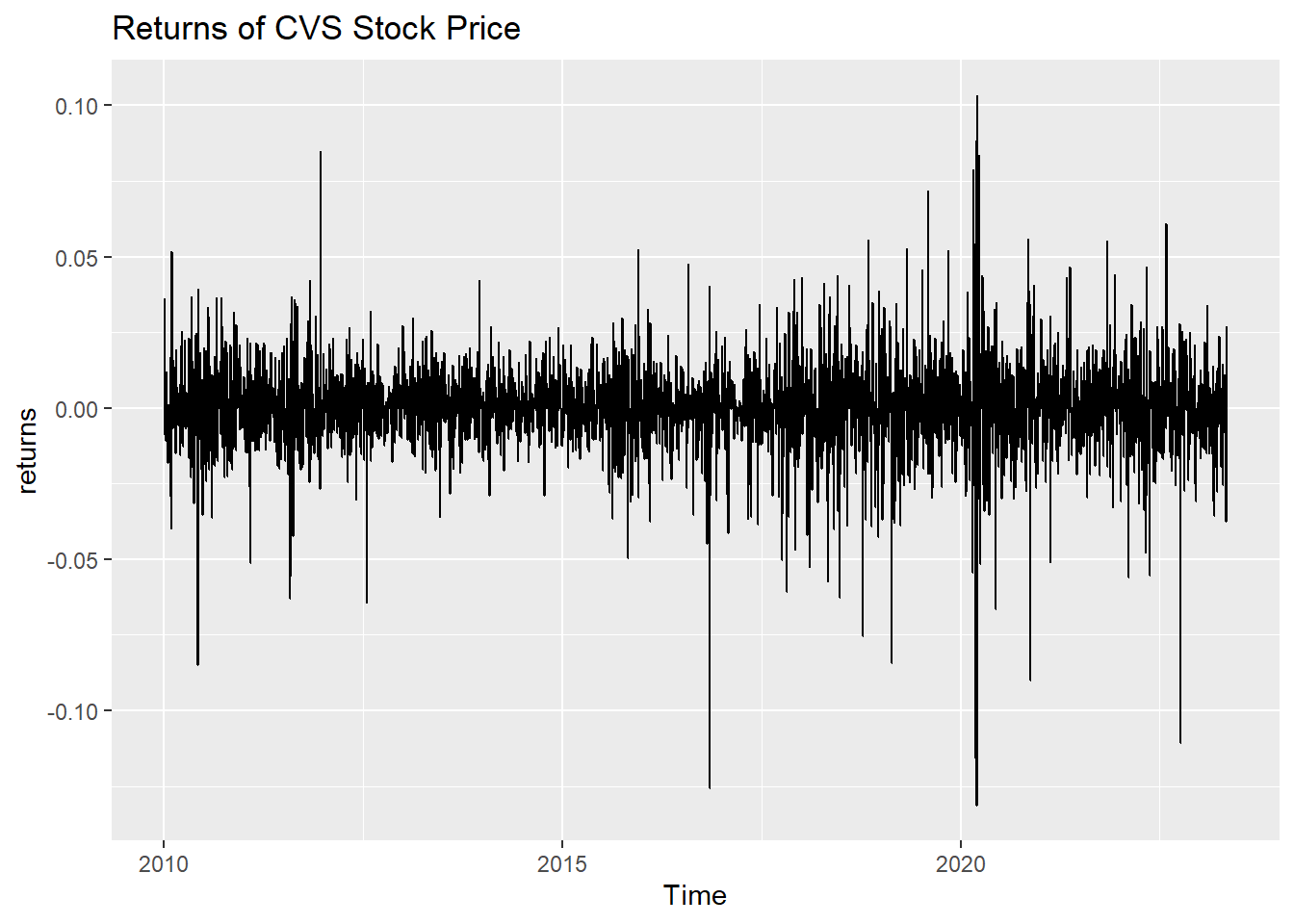
ACF, PACF plots of the returns
Show the code
ggAcf(returns)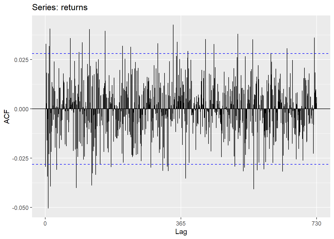
Show the code
ggPacf(returns)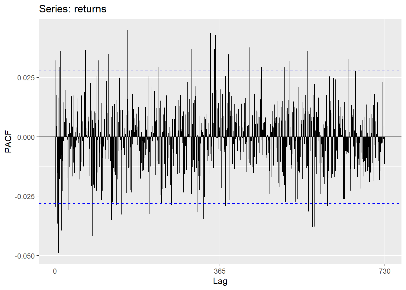
These plots here shows a closer look of ACF and PACF plots, which are weakly stationary.
Show the code
## have a closer look
acf(returns)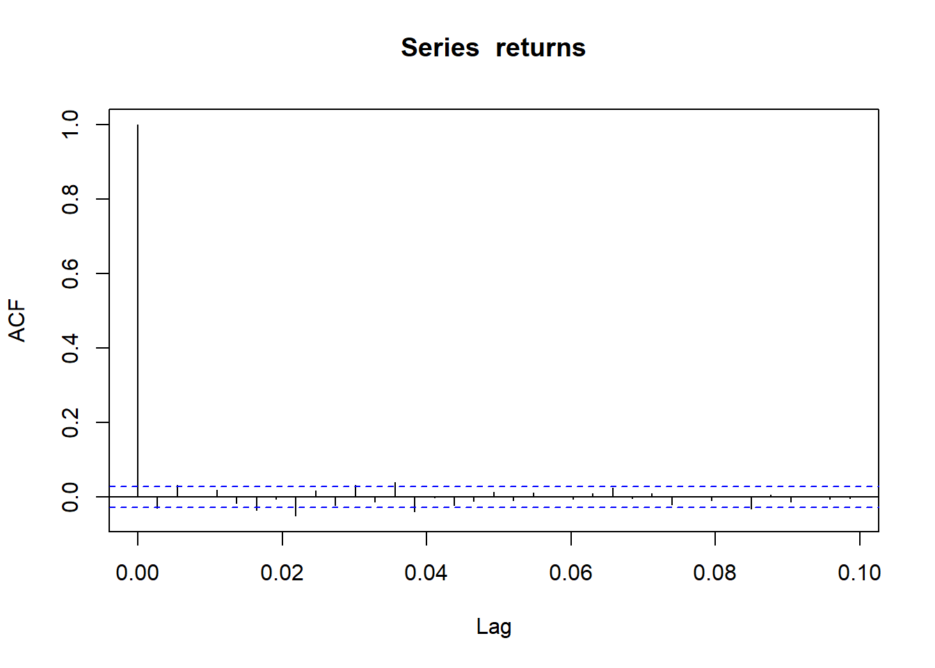
Show the code
pacf(returns)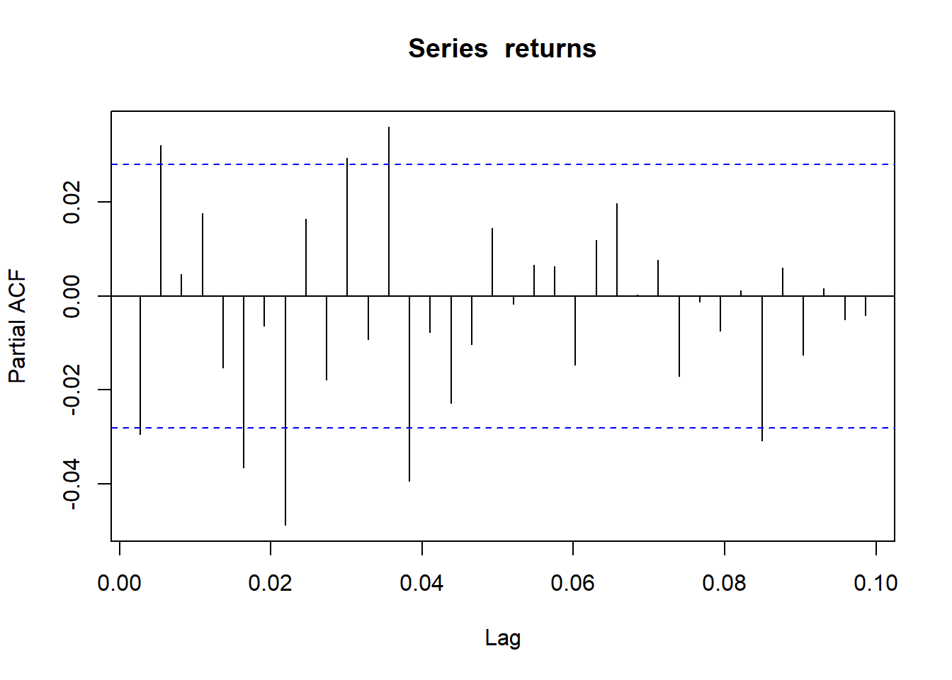
Let’s look at the ACF of absolute values of the returns and squared values. We can see clear correlation in both plots. This correlation is comming from the correlation in conditional variation.
Show the code
acf(abs(returns))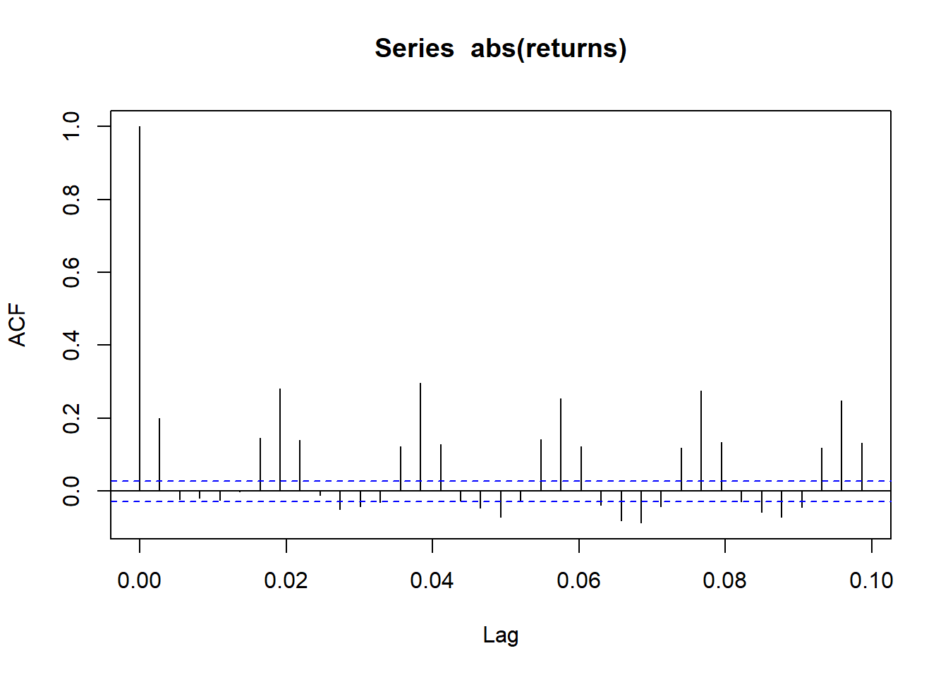
Show the code
acf(returns^2)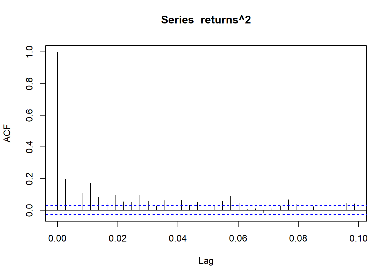
Model Fitting Method
There are two ways we can think of fitting the models. First is that we fit the ARIMA model first and fit a GARCH model for the residual. Second method will be fitting a GARRCH model for the squared returns directly.
Model Fitting Method 1: GARCH(p,q) model fittin
ArchTest
Show the code
library(FinTS)
Attaching package: 'FinTS'The following object is masked from 'package:forecast':
AcfShow the code
ArchTest(returns, lags=1, demean=TRUE)
    ARCH LM-test; Null hypothesis: no ARCH effects

data:  returns
Chi-squared = 185.64, df = 1, p-value < 2.2e-16
Because the p-value is < 0.05, we reject the null hypothesis and conclude the presence of ARCH(1) effects.
Fitting an ARIMA model
Let’s fit the ARIMA model first.
Show the code
ARIMA.c=function(p1,p2,q1,q2,data){
temp=c()
d=1
i=1
temp= data.frame()
ls=matrix(rep(NA,6*50),nrow=50)


for (p in p1:p2)#
{
  for(q in q1:q2)#
  {
    for(d in 0:2)#
    {

      if(p+d+q<=6)
      {

        model<- Arima(data,order=c(p,d,q))
        ls[i,]= c(p,d,q,model$aic,model$bic,model$aicc)
        i=i+1


      }

    }
  }
}


temp= as.data.frame(ls)
names(temp)= c("p","d","q","AIC","BIC","AICc")

temp
}
Show the code
#na.omit(log(bts)))
output <- ARIMA.c(0,2,0,2,data=log(CVS_ts))
output
p d q AIC BIC AICc
1 0 0 0 5188.446 5201.428 5188.449
2 0 1 0 -28803.633 -28797.142 -28803.632
3 0 2 0 -25285.070 -25278.580 -25285.069
4 0 0 1 -1368.727 -1349.255 -1368.722
5 0 1 1 -28805.510 -28792.528 -28805.507
6 0 2 1 -28787.667 -28774.686 -28787.665
7 0 0 2 -6872.140 -6846.177 -6872.132
8 0 1 2 -28808.808 -28789.336 -28808.803
9 0 2 2 -28789.562 -28770.090 -28789.557
10 1 0 0 -28798.783 -28779.311 -28798.778
11 1 1 0 -28805.766 -28792.784 -28805.763
12 1 2 0 -26889.073 -26876.092 -26889.070
13 1 0 1 -28800.561 -28774.598 -28800.553
14 1 1 1 -28807.187 -28787.715 -28807.182
15 1 2 1 -28789.827 -28770.356 -28789.822
16 1 0 2 -28803.967 -28771.513 -28803.955
17 1 1 2 -28806.786 -28780.823 -28806.778
18 1 2 2 -28785.523 -28759.561 -28785.514
19 2 0 0 -28800.794 -28774.831 -28800.786
20 2 1 0 -28808.910 -28789.438 -28808.905
21 2 2 0 -27443.617 -27424.146 -27443.612
22 2 0 1 -28802.321 -28769.867 -28802.308
23 2 1 1 -28806.931 -28780.969 -28806.923
24 2 2 1 -28792.937 -28766.976 -28792.929
25 2 0 2 -28796.612 -28757.666 -28796.594
26 2 1 2 -28804.961 -28772.508 -28804.949
27 2 2 2 -28787.125 -28754.673 -28787.113
28 NA NA NA NA NA NA
29 NA NA NA NA NA NA
30 NA NA NA NA NA NA
31 NA NA NA NA NA NA
32 NA NA NA NA NA NA
33 NA NA NA NA NA NA
34 NA NA NA NA NA NA
35 NA NA NA NA NA NA
36 NA NA NA NA NA NA
37 NA NA NA NA NA NA
38 NA NA NA NA NA NA
39 NA NA NA NA NA NA
40 NA NA NA NA NA NA
41 NA NA NA NA NA NA
42 NA NA NA NA NA NA
43 NA NA NA NA NA NA
44 NA NA NA NA NA NA
45 NA NA NA NA NA NA
46 NA NA NA NA NA NA
47 NA NA NA NA NA NA
48 NA NA NA NA NA NA
49 NA NA NA NA NA NA
50 NA NA NA NA NA NAShow the code
output[which.min(output$AIC),] p d q AIC BIC AICc
20 2 1 0 -28808.91 -28789.44 -28808.91Show the code
output[which.min(output$BIC),] p d q AIC BIC AICc
2 0 1 0 -28803.63 -28797.14 -28803.63Show the code
output[which.min(output$AICc),] p d q AIC BIC AICc
20 2 1 0 -28808.91 -28789.44 -28808.91Show the code
auto.arima(log(CVS_ts))Series: log(CVS_ts)
ARIMA(3,1,0)
Coefficients:
ar1 ar2 ar3
-0.0284 0.0327 0.0050
s.e. 0.0143 0.0143 0.0144
sigma^2 = 0.0001576: log likelihood = 14407.52
AIC=-28807.03 AICc=-28807.02 BIC=-28781.07Show the code
data=log(CVS_ts)
sarima(data, 0,1,0) #has lower BIC
initial value -4.377149
iter 1 value -4.377149
final value -4.377149
converged
initial value -4.377149
iter 1 value -4.377149
final value -4.377149
converged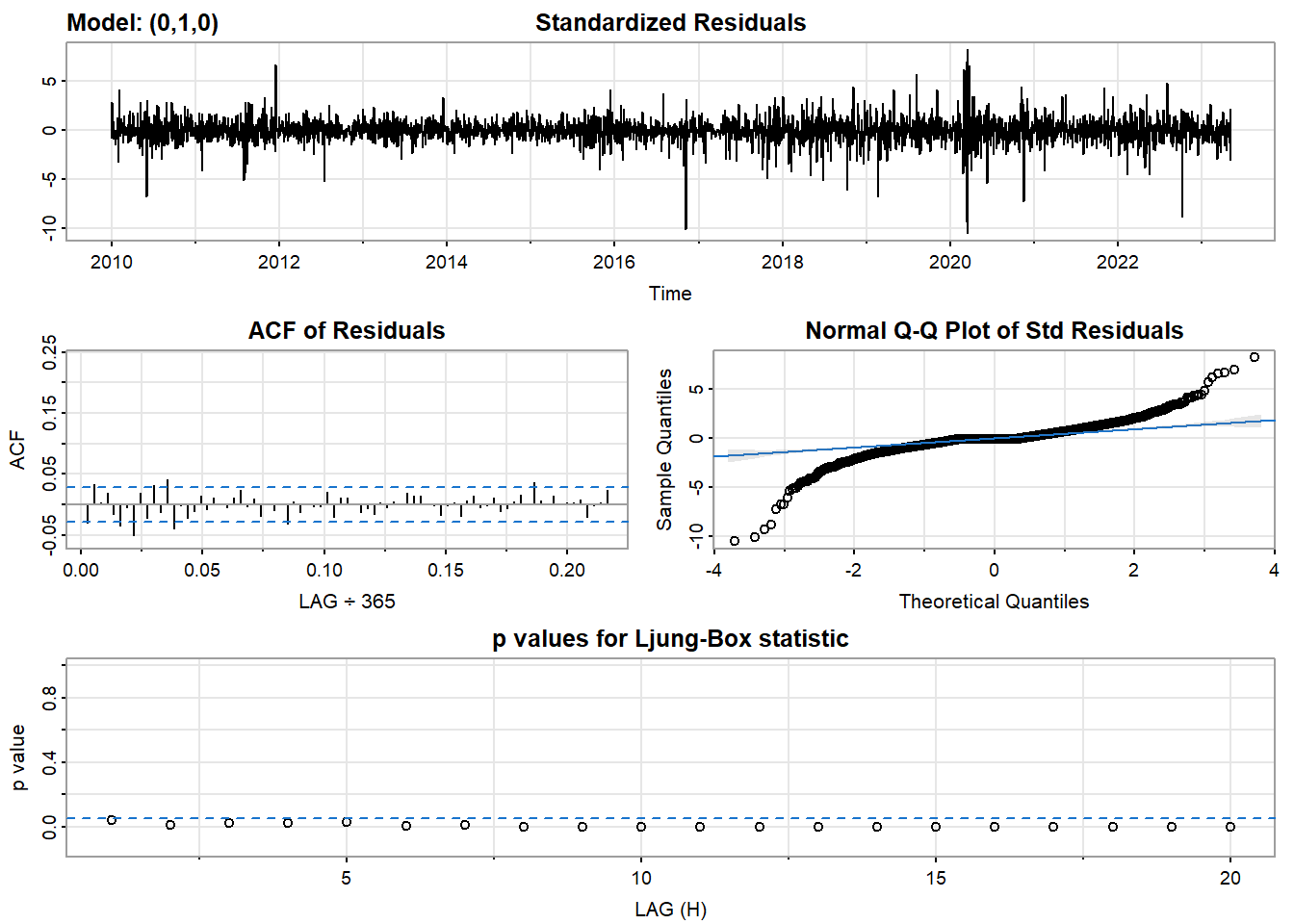
$fit

Call:
arima(x = xdata, order = c(p, d, q), seasonal = list(order = c(P, D, Q), period = S),
    xreg = constant, transform.pars = trans, fixed = fixed, optim.control = list(trace = trc,
        REPORT = 1, reltol = tol))

Coefficients:
      constant
         2e-04
s.e.     2e-04

sigma^2 estimated as 0.0001578:  log likelihood = 14403.53,  aic = -28803.05

$degrees_of_freedom
[1] 4868

$ttable
         Estimate    SE t.value p.value
constant    2e-04 2e-04  1.1879  0.2349

$AIC
[1] -5.915599

$AICc
[1] -5.915599

$BIC
[1] -5.912933
I’m going to choose ARIMA(0,1,0) because it has the lowest BIC and the hole model diagnostics are the same.
Fit the GARCH model
First fit the ARIMA model and fitting a GARCH model to the residuals of the ARIMA model.
Show the code
arima.fit<-Arima(data,order=c(0,1,0),include.drift = TRUE)
arima.res<-arima.fit$residuals

acf(arima.res)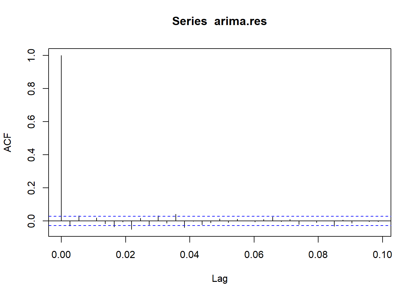
Show the code
acf(arima.res^2) #clear correlation 1,3,4,5,6,7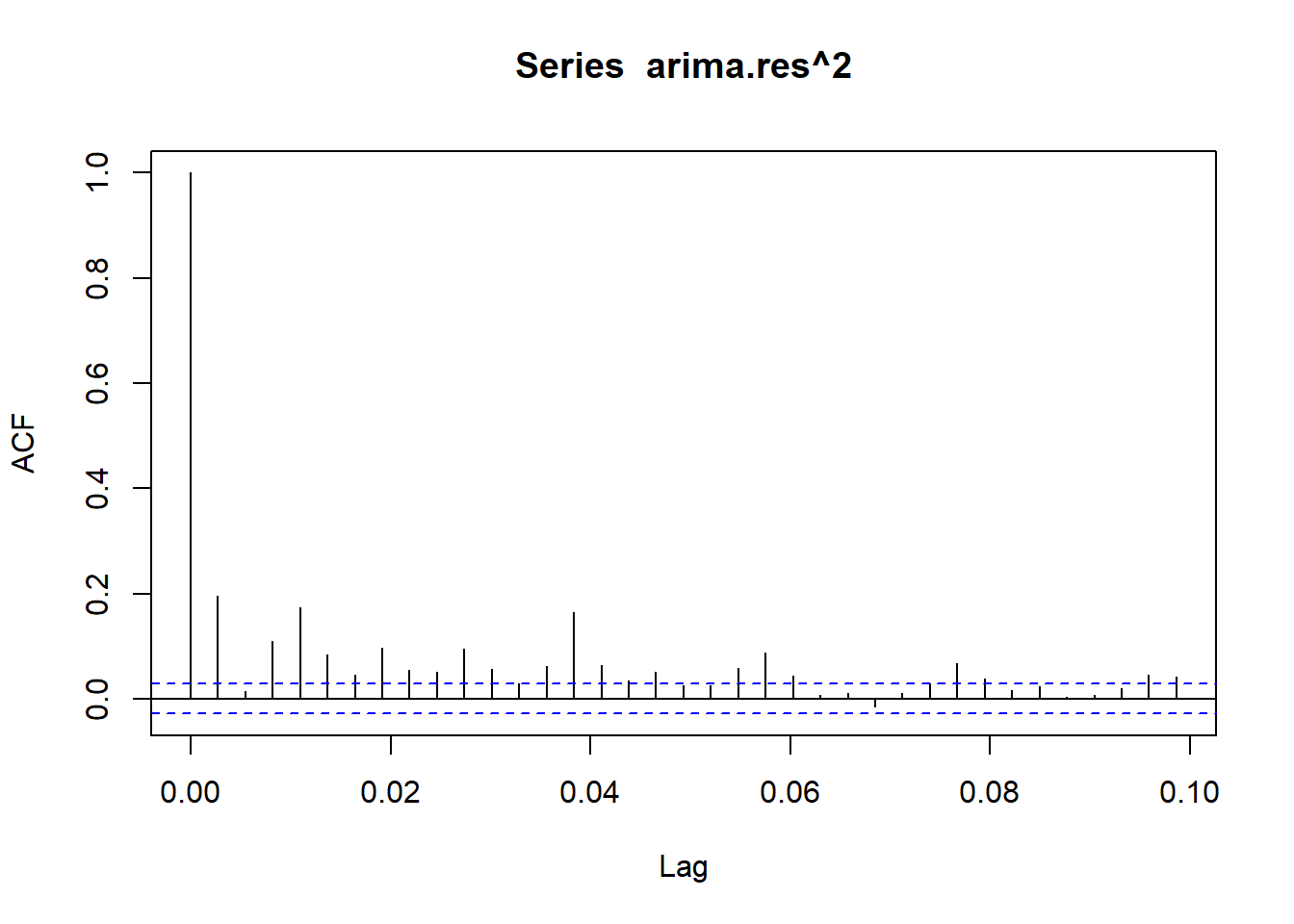
Show the code
pacf(arima.res^2) #1,3,4,7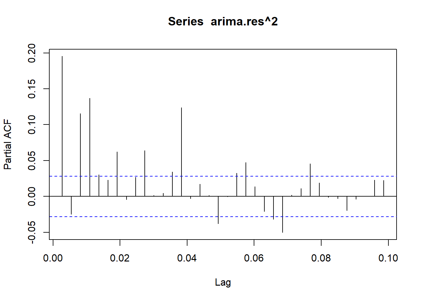
Show the code
model <- list() ## set counter
cc <- 1
for (p in 1:7) {
  for (q in 1:7) {

model[[cc]] <- garch(arima.res,order=c(q,p),trace=F)
cc <- cc + 1
}
}

## get AIC values for model evaluation
GARCH_AIC <- sapply(model, AIC) ## model with lowest AIC is the best
which(GARCH_AIC == min(GARCH_AIC))
[1] 7Show the code
model[[which(GARCH_AIC == min(GARCH_AIC))]]
Call:
garch(x = arima.res, order = c(q, p), trace = F)

Coefficient(s):
       a0         a1         b1         b2         b3         b4         b5
9.954e-06  1.886e-01  1.034e-08  7.187e-02  5.132e-03  7.429e-02  1.092e-01
       b6         b7
2.588e-01  2.296e-01
Show the code
summary(garchFit(~garch(1,3), arima.res,trace = F))
Title:
 GARCH Modelling

Call:
 garchFit(formula = ~garch(1, 3), data = arima.res, trace = F)

Mean and Variance Equation:
 data ~ garch(1, 3)
<environment: 0x000001953db8c950>
 [data = arima.res]

Conditional Distribution:
 norm

Coefficient(s):
        mu       omega      alpha1       beta1       beta2       beta3
6.5984e-06  7.7096e-06  1.1708e-01  1.0000e-08  6.0691e-01  2.3160e-01

Std. Errors:
 based on Hessian

Error Analysis:
        Estimate  Std. Error  t value Pr(>|t|)
mu     6.598e-06   1.553e-04    0.042  0.96612
omega  7.710e-06   2.105e-06    3.663  0.00025 ***
alpha1 1.171e-01   2.496e-02    4.690 2.73e-06 ***
beta1  1.000e-08   2.671e-01    0.000  1.00000
beta2  6.069e-01   8.319e-02    7.296 2.97e-13 ***
beta3  2.316e-01   1.851e-01    1.251  0.21076
---
Signif. codes:  0 '***' 0.001 '**' 0.01 '*' 0.05 '.' 0.1 ' ' 1

Log Likelihood:
 14765.65    normalized:  3.031961

Description:
 Sat May  6 19:21:46 2023 by user: yujia


Standardised Residuals Tests:
                                Statistic p-Value
 Jarque-Bera Test   R    Chi^2  13768.98  0
 Shapiro-Wilk Test  R    W      0.8849537 0
 Ljung-Box Test     R    Q(10)  16.40464  0.08862022
 Ljung-Box Test     R    Q(15)  21.02519  0.1360265
 Ljung-Box Test     R    Q(20)  24.48768  0.2217382
 Ljung-Box Test     R^2  Q(10)  12.52544  0.251428
 Ljung-Box Test     R^2  Q(15)  23.88171  0.0671297
 Ljung-Box Test     R^2  Q(20)  37.28578  0.01081188
 LM Arch Test       R    TR^2   13.95831  0.3033781

Information Criterion Statistics:
      AIC       BIC       SIC      HQIC
-6.061457 -6.053460 -6.061460 -6.058651
beta 3 is not significant. So I’m going to try GARCH(1,1) and GARCH(1,2).
Show the code
summary(garchFit(~garch(1,2), arima.res,trace = F))
Title:
 GARCH Modelling

Call:
 garchFit(formula = ~garch(1, 2), data = arima.res, trace = F)

Mean and Variance Equation:
 data ~ garch(1, 2)
<environment: 0x000001953da0c198>
 [data = arima.res]

Conditional Distribution:
 norm

Coefficient(s):
        mu       omega      alpha1       beta1       beta2
6.5984e-06  6.6528e-06  9.7007e-02  1.5783e-01  7.0639e-01

Std. Errors:
 based on Hessian

Error Analysis:
        Estimate  Std. Error  t value Pr(>|t|)
mu     6.598e-06   1.563e-04    0.042    0.966
omega  6.653e-06   1.450e-06    4.588 4.48e-06 ***
alpha1 9.701e-02   1.186e-02    8.183 2.22e-16 ***
beta1  1.578e-01   3.856e-02    4.092 4.27e-05 ***
beta2  7.064e-01   3.909e-02   18.073  < 2e-16 ***
---
Signif. codes:  0 '***' 0.001 '**' 0.01 '*' 0.05 '.' 0.1 ' ' 1

Log Likelihood:
 14757.81    normalized:  3.03035

Description:
 Sat May  6 19:21:48 2023 by user: yujia


Standardised Residuals Tests:
                                Statistic p-Value
 Jarque-Bera Test   R    Chi^2  13277.74  0
 Shapiro-Wilk Test  R    W      0.885234  0
 Ljung-Box Test     R    Q(10)  16.12467  0.0961187
 Ljung-Box Test     R    Q(15)  20.97592  0.1376006
 Ljung-Box Test     R    Q(20)  24.21644  0.2330654
 Ljung-Box Test     R^2  Q(10)  13.41383  0.2014453
 Ljung-Box Test     R^2  Q(15)  24.89258  0.05140473
 Ljung-Box Test     R^2  Q(20)  38.30603  0.00812319
 LM Arch Test       R    TR^2   14.54909  0.2670261

Information Criterion Statistics:
      AIC       BIC       SIC      HQIC
-6.058647 -6.051983 -6.058649 -6.056308
Show the code
summary(garchFit(~garch(1,1), arima.res,trace = F))
Title:
 GARCH Modelling

Call:
 garchFit(formula = ~garch(1, 1), data = arima.res, trace = F)

Mean and Variance Equation:
 data ~ garch(1, 1)
<environment: 0x000001953bee5b98>
 [data = arima.res]

Conditional Distribution:
 norm

Coefficient(s):
        mu       omega      alpha1       beta1
6.5984e-06  3.2972e-06  5.0081e-02  9.3069e-01

Std. Errors:
 based on Hessian

Error Analysis:
        Estimate  Std. Error  t value Pr(>|t|)
mu     6.598e-06   1.578e-04    0.042    0.967
omega  3.297e-06   7.454e-07    4.423 9.72e-06 ***
alpha1 5.008e-02   6.617e-03    7.569 3.77e-14 ***
beta1  9.307e-01   9.836e-03   94.616  < 2e-16 ***
---
Signif. codes:  0 '***' 0.001 '**' 0.01 '*' 0.05 '.' 0.1 ' ' 1

Log Likelihood:
 14736.05    normalized:  3.025883

Description:
 Sat May  6 19:21:49 2023 by user: yujia


Standardised Residuals Tests:
                                Statistic p-Value
 Jarque-Bera Test   R    Chi^2  15641.72  0
 Shapiro-Wilk Test  R    W      0.8830468 0
 Ljung-Box Test     R    Q(10)  15.06102  0.1298529
 Ljung-Box Test     R    Q(15)  19.81811  0.1790219
 Ljung-Box Test     R    Q(20)  23.49551  0.2651236
 Ljung-Box Test     R^2  Q(10)  14.27008  0.1610251
 Ljung-Box Test     R^2  Q(15)  24.61863  0.05530551
 Ljung-Box Test     R^2  Q(20)  35.98932  0.01542563
 LM Arch Test       R    TR^2   16.29535  0.1780798

Information Criterion Statistics:
      AIC       BIC       SIC      HQIC
-6.050124 -6.044793 -6.050125 -6.048253
Since all the models has similar AIC ,BIC values, I would go with GARCH(1,1) which all the coefficients are significant.
Final Model
Show the code
summary(arima.fit<-Arima(data,order=c(0,1,0),include.drift = TRUE))Series: data
ARIMA(0,1,0) with drift
Coefficients:
drift
2e-04
s.e. 2e-04
sigma^2 = 0.0001578: log likelihood = 14403.53
AIC=-28803.05 AICc=-28803.05 BIC=-28790.07
Training set error measures:
ME RMSE MAE MPE MAPE
Training set 6.598419e-07 0.01255991 0.007331295 -0.0001026668 0.1847525
MASE ACF1
Training set 0.03791226 -0.0294275Show the code
summary(final.fit <- garchFit(~garch(1,1), arima.res,trace = F))
Title:
 GARCH Modelling

Call:
 garchFit(formula = ~garch(1, 1), data = arima.res, trace = F)

Mean and Variance Equation:
 data ~ garch(1, 1)
<environment: 0x000001953d506130>
 [data = arima.res]

Conditional Distribution:
 norm

Coefficient(s):
        mu       omega      alpha1       beta1
6.5984e-06  3.2972e-06  5.0081e-02  9.3069e-01

Std. Errors:
 based on Hessian

Error Analysis:
        Estimate  Std. Error  t value Pr(>|t|)
mu     6.598e-06   1.578e-04    0.042    0.967
omega  3.297e-06   7.454e-07    4.423 9.72e-06 ***
alpha1 5.008e-02   6.617e-03    7.569 3.77e-14 ***
beta1  9.307e-01   9.836e-03   94.616  < 2e-16 ***
---
Signif. codes:  0 '***' 0.001 '**' 0.01 '*' 0.05 '.' 0.1 ' ' 1

Log Likelihood:
 14736.05    normalized:  3.025883

Description:
 Sat May  6 19:21:51 2023 by user: yujia


Standardised Residuals Tests:
                                Statistic p-Value
 Jarque-Bera Test   R    Chi^2  15641.72  0
 Shapiro-Wilk Test  R    W      0.8830468 0
 Ljung-Box Test     R    Q(10)  15.06102  0.1298529
 Ljung-Box Test     R    Q(15)  19.81811  0.1790219
 Ljung-Box Test     R    Q(20)  23.49551  0.2651236
 Ljung-Box Test     R^2  Q(10)  14.27008  0.1610251
 Ljung-Box Test     R^2  Q(15)  24.61863  0.05530551
 Ljung-Box Test     R^2  Q(20)  35.98932  0.01542563
 LM Arch Test       R    TR^2   16.29535  0.1780798

Information Criterion Statistics:
      AIC       BIC       SIC      HQIC
-6.050124 -6.044793 -6.050125 -6.048253
Forecast
Show the code
predict(final.fit, n.ahead = 100, plot=TRUE)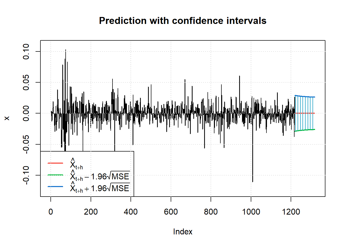
    meanForecast  meanError standardDeviation lowerInterval upperInterval
1   6.598419e-06 0.01476927        0.01476927   -0.02894064    0.02895384
2   6.598419e-06 0.01473888        0.01473888   -0.02888108    0.02889428
3   6.598419e-06 0.01470902        0.01470902   -0.02882255    0.02883574
4   6.598419e-06 0.01467967        0.01467967   -0.02876502    0.02877822
5   6.598419e-06 0.01465083        0.01465083   -0.02870849    0.02872169
6   6.598419e-06 0.01462248        0.01462248   -0.02865294    0.02866614
7   6.598419e-06 0.01459463        0.01459463   -0.02859835    0.02861155
8   6.598419e-06 0.01456726        0.01456726   -0.02854471    0.02855791
9   6.598419e-06 0.01454037        0.01454037   -0.02849200    0.02850520
10  6.598419e-06 0.01451395        0.01451395   -0.02844022    0.02845341
11  6.598419e-06 0.01448799        0.01448799   -0.02838933    0.02840253
12  6.598419e-06 0.01446248        0.01446248   -0.02833934    0.02835253
13  6.598419e-06 0.01443742        0.01443742   -0.02829022    0.02830342
14  6.598419e-06 0.01441279        0.01441279   -0.02824196    0.02825516
15  6.598419e-06 0.01438861        0.01438861   -0.02819455    0.02820775
16  6.598419e-06 0.01436484        0.01436484   -0.02814797    0.02816117
17  6.598419e-06 0.01434150        0.01434150   -0.02810222    0.02811541
18  6.598419e-06 0.01431856        0.01431856   -0.02805727    0.02807047
19  6.598419e-06 0.01429603        0.01429603   -0.02801312    0.02802631
20  6.598419e-06 0.01427391        0.01427391   -0.02796974    0.02798294
21  6.598419e-06 0.01425217        0.01425217   -0.02792714    0.02794033
22  6.598419e-06 0.01423082        0.01423082   -0.02788529    0.02789849
23  6.598419e-06 0.01420984        0.01420984   -0.02784418    0.02785738
24  6.598419e-06 0.01418924        0.01418924   -0.02780381    0.02781701
25  6.598419e-06 0.01416901        0.01416901   -0.02776416    0.02777735
26  6.598419e-06 0.01414914        0.01414914   -0.02772521    0.02773840
27  6.598419e-06 0.01412962        0.01412962   -0.02768696    0.02770015
28  6.598419e-06 0.01411046        0.01411046   -0.02764939    0.02766259
29  6.598419e-06 0.01409163        0.01409163   -0.02761249    0.02762569
30  6.598419e-06 0.01407315        0.01407315   -0.02757626    0.02758946
31  6.598419e-06 0.01405499        0.01405499   -0.02754068    0.02755387
32  6.598419e-06 0.01403716        0.01403716   -0.02750573    0.02751893
33  6.598419e-06 0.01401965        0.01401965   -0.02747142    0.02748462
34  6.598419e-06 0.01400246        0.01400246   -0.02743772    0.02745092
35  6.598419e-06 0.01398558        0.01398558   -0.02740463    0.02741783
36  6.598419e-06 0.01396900        0.01396900   -0.02737214    0.02738534
37  6.598419e-06 0.01395272        0.01395272   -0.02734024    0.02735343
38  6.598419e-06 0.01393674        0.01393674   -0.02730891    0.02732210
39  6.598419e-06 0.01392104        0.01392104   -0.02727815    0.02729134
40  6.598419e-06 0.01390563        0.01390563   -0.02724794    0.02726114
41  6.598419e-06 0.01389050        0.01389050   -0.02721829    0.02723149
42  6.598419e-06 0.01387565        0.01387565   -0.02718917    0.02720237
43  6.598419e-06 0.01386106        0.01386106   -0.02716059    0.02717379
44  6.598419e-06 0.01384675        0.01384675   -0.02713252    0.02714572
45  6.598419e-06 0.01383269        0.01383269   -0.02710497    0.02711817
46  6.598419e-06 0.01381888        0.01381888   -0.02707792    0.02709111
47  6.598419e-06 0.01380533        0.01380533   -0.02705136    0.02706456
48  6.598419e-06 0.01379203        0.01379203   -0.02702529    0.02703848
49  6.598419e-06 0.01377897        0.01377897   -0.02699969    0.02701289
50  6.598419e-06 0.01376615        0.01376615   -0.02697456    0.02698776
51  6.598419e-06 0.01375357        0.01375357   -0.02694990    0.02696309
52  6.598419e-06 0.01374121        0.01374121   -0.02692568    0.02693888
53  6.598419e-06 0.01372908        0.01372908   -0.02690191    0.02691511
54  6.598419e-06 0.01371718        0.01371718   -0.02687858    0.02689177
55  6.598419e-06 0.01370549        0.01370549   -0.02685567    0.02686887
56  6.598419e-06 0.01369402        0.01369402   -0.02683319    0.02684639
57  6.598419e-06 0.01368276        0.01368276   -0.02681112    0.02682432
58  6.598419e-06 0.01367171        0.01367171   -0.02678946    0.02680265
59  6.598419e-06 0.01366086        0.01366086   -0.02676819    0.02678139
60  6.598419e-06 0.01365021        0.01365021   -0.02674732    0.02676052
61  6.598419e-06 0.01363976        0.01363976   -0.02672684    0.02674003
62  6.598419e-06 0.01362950        0.01362950   -0.02670673    0.02671993
63  6.598419e-06 0.01361943        0.01361943   -0.02668700    0.02670019
64  6.598419e-06 0.01360955        0.01360955   -0.02666763    0.02668082
65  6.598419e-06 0.01359985        0.01359985   -0.02664862    0.02666181
66  6.598419e-06 0.01359033        0.01359033   -0.02662996    0.02664315
67  6.598419e-06 0.01358099        0.01358099   -0.02661164    0.02662484
68  6.598419e-06 0.01357182        0.01357182   -0.02659367    0.02660687
69  6.598419e-06 0.01356282        0.01356282   -0.02657603    0.02658923
70  6.598419e-06 0.01355398        0.01355398   -0.02655872    0.02657192
71  6.598419e-06 0.01354532        0.01354532   -0.02654173    0.02655493
72  6.598419e-06 0.01353681        0.01353681   -0.02652506    0.02653826
73  6.598419e-06 0.01352846        0.01352846   -0.02650870    0.02652189
74  6.598419e-06 0.01352027        0.01352027   -0.02649264    0.02650583
75  6.598419e-06 0.01351223        0.01351223   -0.02647688    0.02649008
76  6.598419e-06 0.01350434        0.01350434   -0.02646141    0.02647461
77  6.598419e-06 0.01349659        0.01349659   -0.02644624    0.02645943
78  6.598419e-06 0.01348899        0.01348899   -0.02643135    0.02644454
79  6.598419e-06 0.01348154        0.01348154   -0.02641673    0.02642993
80  6.598419e-06 0.01347422        0.01347422   -0.02640239    0.02641559
81  6.598419e-06 0.01346704        0.01346704   -0.02638831    0.02640151
82  6.598419e-06 0.01345999        0.01345999   -0.02637450    0.02638770
83  6.598419e-06 0.01345308        0.01345308   -0.02636095    0.02637415
84  6.598419e-06 0.01344629        0.01344629   -0.02634765    0.02636085
85  6.598419e-06 0.01343964        0.01343964   -0.02633461    0.02634780
86  6.598419e-06 0.01343310        0.01343310   -0.02632180    0.02633500
87  6.598419e-06 0.01342669        0.01342669   -0.02630924    0.02632243
88  6.598419e-06 0.01342040        0.01342040   -0.02629691    0.02631011
89  6.598419e-06 0.01341423        0.01341423   -0.02628481    0.02629801
90  6.598419e-06 0.01340818        0.01340818   -0.02627294    0.02628614
91  6.598419e-06 0.01340223        0.01340223   -0.02626130    0.02627449
92  6.598419e-06 0.01339640        0.01339640   -0.02624987    0.02626306
93  6.598419e-06 0.01339068        0.01339068   -0.02623866    0.02625185
94  6.598419e-06 0.01338507        0.01338507   -0.02622765    0.02624085
95  6.598419e-06 0.01337956        0.01337956   -0.02621686    0.02623006
96  6.598419e-06 0.01337416        0.01337416   -0.02620627    0.02621946
97  6.598419e-06 0.01336885        0.01336885   -0.02619587    0.02620907
98  6.598419e-06 0.01336365        0.01336365   -0.02618568    0.02619887
99  6.598419e-06 0.01335855        0.01335855   -0.02617567    0.02618887
100 6.598419e-06 0.01335354        0.01335354   -0.02616586    0.02617905
Volatality plot
Show the code
ht <- final.fit@h.t

data= data.frame(ht,CVS_df$Date)
ggplot(data, aes(y = ht, x = CVS_df$Date)) + geom_line(col = '#ff9933') + ylab('Conditional Variance') + xlab('Date')+ggtitle("Volatility plot of CVS Stock Price")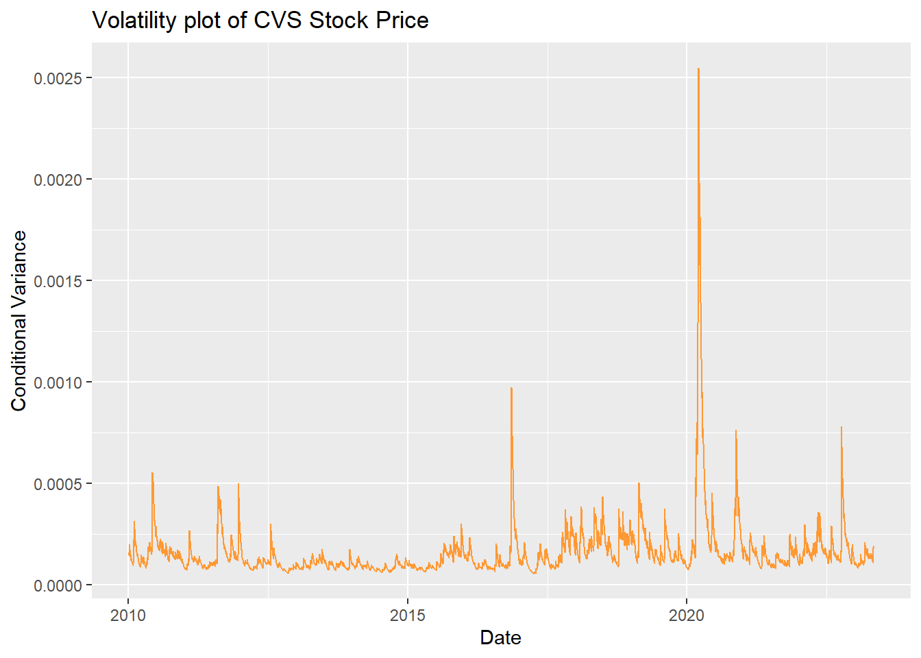
There’s obvious volatality 2016 that’s when U.S. presidential election and potential changes to healthcare policy, then even more volatality in 2020 because of COVID.
Model Fitting Method 2: GARCH(p,q) model fitting
Here is going to fit a GARCH model directly.
Show the code
pacf(returns^2) #p=1,3,4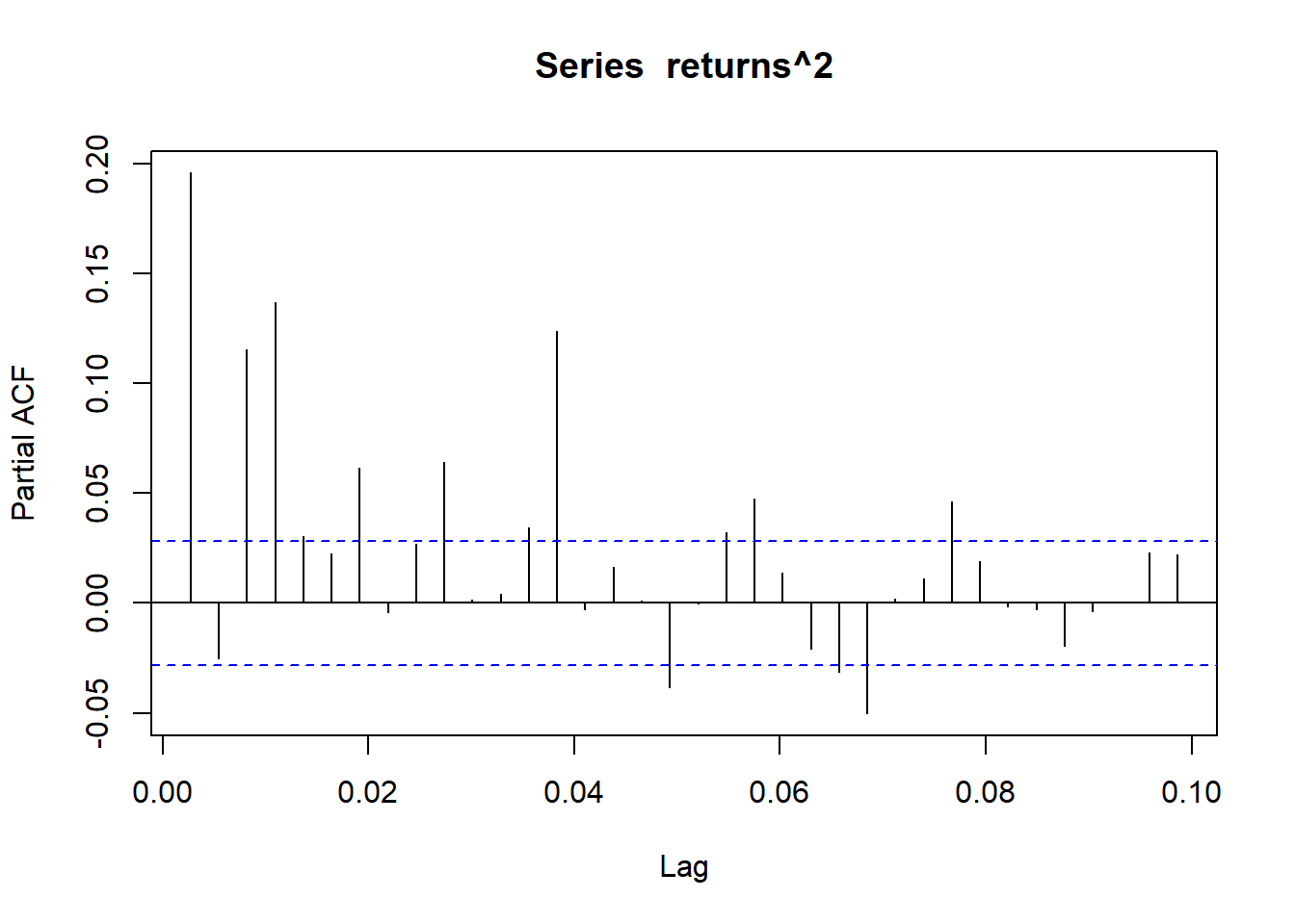
Show the code
model <- list() ## set counter
cc <- 1
for (p in 1:7) {
  for (q in 1:7) {

model[[cc]] <- garch(returns,order=c(q,p),trace=F)
cc <- cc + 1
}
}

## get AIC values for model evaluation
GARCH_AIC <- sapply(model, AIC) ## model with lowest AIC is the best
which(GARCH_AIC == min(GARCH_AIC))
[1] 7Show the code
model[[which(GARCH_AIC == min(GARCH_AIC))]]
Call:
garch(x = returns, order = c(q, p), trace = F)

Coefficient(s):
       a0         a1         b1         b2         b3         b4         b5
9.365e-06  1.889e-01  3.534e-03  7.306e-02  1.971e-09  7.335e-02  1.122e-01
       b6         b7
2.612e-01  2.304e-01
Show the code
summary(garchFit(~garch(1,3), returns,trace = F))
Title:
 GARCH Modelling

Call:
 garchFit(formula = ~garch(1, 3), data = returns, trace = F)

Mean and Variance Equation:
 data ~ garch(1, 3)
<environment: 0x000001953daa83a8>
 [data = returns]

Conditional Distribution:
 norm

Coefficient(s):
        mu       omega      alpha1       beta1       beta2       beta3
3.5413e-04  7.7412e-06  1.1746e-01  1.0000e-08  6.0492e-01  2.3303e-01

Std. Errors:
 based on Hessian

Error Analysis:
        Estimate  Std. Error  t value Pr(>|t|)
mu     3.541e-04   1.554e-04    2.279 0.022696 *
omega  7.741e-06   2.103e-06    3.681 0.000232 ***
alpha1 1.175e-01   2.465e-02    4.765 1.89e-06 ***
beta1  1.000e-08   2.635e-01    0.000 1.000000
beta2  6.049e-01   8.425e-02    7.180 6.97e-13 ***
beta3  2.330e-01   1.812e-01    1.286 0.198408
---
Signif. codes:  0 '***' 0.001 '**' 0.01 '*' 0.05 '.' 0.1 ' ' 1

Log Likelihood:
 14762.73    normalized:  3.031983

Description:
 Sat May  6 19:21:54 2023 by user: yujia


Standardised Residuals Tests:
                                Statistic p-Value
 Jarque-Bera Test   R    Chi^2  13757.84  0
 Shapiro-Wilk Test  R    W      0.8853728 0
 Ljung-Box Test     R    Q(10)  16.46796  0.08699736
 Ljung-Box Test     R    Q(15)  21.05861  0.1349671
 Ljung-Box Test     R    Q(20)  24.53261  0.2199005
 Ljung-Box Test     R^2  Q(10)  12.43878  0.2567628
 Ljung-Box Test     R^2  Q(15)  23.71456  0.07010195
 Ljung-Box Test     R^2  Q(20)  37.0202   0.01163694
 LM Arch Test       R    TR^2   13.88701  0.3079816

Information Criterion Statistics:
      AIC       BIC       SIC      HQIC
-6.061502 -6.053504 -6.061505 -6.058695
Beta 3 is not significant. So I’m going to try GARCH(1,1), GARCH(2,2), GARCH(1,2) and GARCH(2,1)
Show the code
summary(garchFit(~garch(1,1), returns,trace = F)) #all significant
Title:
 GARCH Modelling

Call:
 garchFit(formula = ~garch(1, 1), data = returns, trace = F)

Mean and Variance Equation:
 data ~ garch(1, 1)
<environment: 0x000001953e0d4e60>
 [data = returns]

Conditional Distribution:
 norm

Coefficient(s):
        mu       omega      alpha1       beta1
3.5116e-04  3.2985e-06  5.0176e-02  9.3060e-01

Std. Errors:
 based on Hessian

Error Analysis:
        Estimate  Std. Error  t value Pr(>|t|)
mu     3.512e-04   1.577e-04    2.226    0.026 *
omega  3.298e-06   7.474e-07    4.413 1.02e-05 ***
alpha1 5.018e-02   6.646e-03    7.550 4.37e-14 ***
beta1  9.306e-01   9.880e-03   94.191  < 2e-16 ***
---
Signif. codes:  0 '***' 0.001 '**' 0.01 '*' 0.05 '.' 0.1 ' ' 1

Log Likelihood:
 14733.01    normalized:  3.02588

Description:
 Sat May  6 19:21:55 2023 by user: yujia


Standardised Residuals Tests:
                                Statistic p-Value
 Jarque-Bera Test   R    Chi^2  15608.8   0
 Shapiro-Wilk Test  R    W      0.8834462 0
 Ljung-Box Test     R    Q(10)  15.12868  0.1274403
 Ljung-Box Test     R    Q(15)  19.86589  0.1771381
 Ljung-Box Test     R    Q(20)  23.54299  0.2629252
 Ljung-Box Test     R^2  Q(10)  14.20457  0.1638634
 Ljung-Box Test     R^2  Q(15)  24.50026  0.05707071
 Ljung-Box Test     R^2  Q(20)  35.79802  0.0162434
 LM Arch Test       R    TR^2   16.24371  0.1803268

Information Criterion Statistics:
      AIC       BIC       SIC      HQIC
-6.050116 -6.044784 -6.050118 -6.048245
Show the code
summary(garchFit(~garch(1,2), returns,trace = F)) #all significant
Title:
 GARCH Modelling

Call:
 garchFit(formula = ~garch(1, 2), data = returns, trace = F)

Mean and Variance Equation:
 data ~ garch(1, 2)
<environment: 0x000001953f631e88>
 [data = returns]

Conditional Distribution:
 norm

Coefficient(s):
        mu       omega      alpha1       beta1       beta2
3.4949e-04  6.6517e-06  9.7054e-02  1.5883e-01  7.0537e-01

Std. Errors:
 based on Hessian

Error Analysis:
        Estimate  Std. Error  t value Pr(>|t|)
mu     3.495e-04   1.562e-04    2.237   0.0253 *
omega  6.652e-06   1.451e-06    4.583 4.58e-06 ***
alpha1 9.705e-02   1.189e-02    8.165 2.22e-16 ***
beta1  1.588e-01   3.879e-02    4.094 4.24e-05 ***
beta2  7.054e-01   3.928e-02   17.955  < 2e-16 ***
---
Signif. codes:  0 '***' 0.001 '**' 0.01 '*' 0.05 '.' 0.1 ' ' 1

Log Likelihood:
 14754.64    normalized:  3.030323

Description:
 Sat May  6 19:21:56 2023 by user: yujia


Standardised Residuals Tests:
                                Statistic p-Value
 Jarque-Bera Test   R    Chi^2  13263.95  0
 Shapiro-Wilk Test  R    W      0.885622  0
 Ljung-Box Test     R    Q(10)  16.18024  0.09458772
 Ljung-Box Test     R    Q(15)  21.00404  0.1367002
 Ljung-Box Test     R    Q(20)  24.2514   0.2315831
 Ljung-Box Test     R^2  Q(10)  13.31937  0.2063598
 Ljung-Box Test     R^2  Q(15)  24.71042  0.05397016
 Ljung-Box Test     R^2  Q(20)  38.0359   0.008766562
 LM Arch Test       R    TR^2   14.46658  0.2719102

Information Criterion Statistics:
      AIC       BIC       SIC      HQIC
-6.058593 -6.051928 -6.058595 -6.056254
Show the code
garch.fit1 <- garchFit(~garch(1,1), data = returns, trace = F)
summary(garch.fit1)
Title:
 GARCH Modelling

Call:
 garchFit(formula = ~garch(1, 1), data = returns, trace = F)

Mean and Variance Equation:
 data ~ garch(1, 1)
<environment: 0x000001953e153bc0>
 [data = returns]

Conditional Distribution:
 norm

Coefficient(s):
        mu       omega      alpha1       beta1
3.5116e-04  3.2985e-06  5.0176e-02  9.3060e-01

Std. Errors:
 based on Hessian

Error Analysis:
        Estimate  Std. Error  t value Pr(>|t|)
mu     3.512e-04   1.577e-04    2.226    0.026 *
omega  3.298e-06   7.474e-07    4.413 1.02e-05 ***
alpha1 5.018e-02   6.646e-03    7.550 4.37e-14 ***
beta1  9.306e-01   9.880e-03   94.191  < 2e-16 ***
---
Signif. codes:  0 '***' 0.001 '**' 0.01 '*' 0.05 '.' 0.1 ' ' 1

Log Likelihood:
 14733.01    normalized:  3.02588

Description:
 Sat May  6 19:21:56 2023 by user: yujia


Standardised Residuals Tests:
                                Statistic p-Value
 Jarque-Bera Test   R    Chi^2  15608.8   0
 Shapiro-Wilk Test  R    W      0.8834462 0
 Ljung-Box Test     R    Q(10)  15.12868  0.1274403
 Ljung-Box Test     R    Q(15)  19.86589  0.1771381
 Ljung-Box Test     R    Q(20)  23.54299  0.2629252
 Ljung-Box Test     R^2  Q(10)  14.20457  0.1638634
 Ljung-Box Test     R^2  Q(15)  24.50026  0.05707071
 Ljung-Box Test     R^2  Q(20)  35.79802  0.0162434
 LM Arch Test       R    TR^2   16.24371  0.1803268

Information Criterion Statistics:
      AIC       BIC       SIC      HQIC
-6.050116 -6.044784 -6.050118 -6.048245
Show the code
garch.fit11<- garch(returns,order=c(1,1),trace=F)
checkresiduals(garch.fit11)
Warning in modeldf.default(object): Could not find appropriate degrees of
freedom for this model.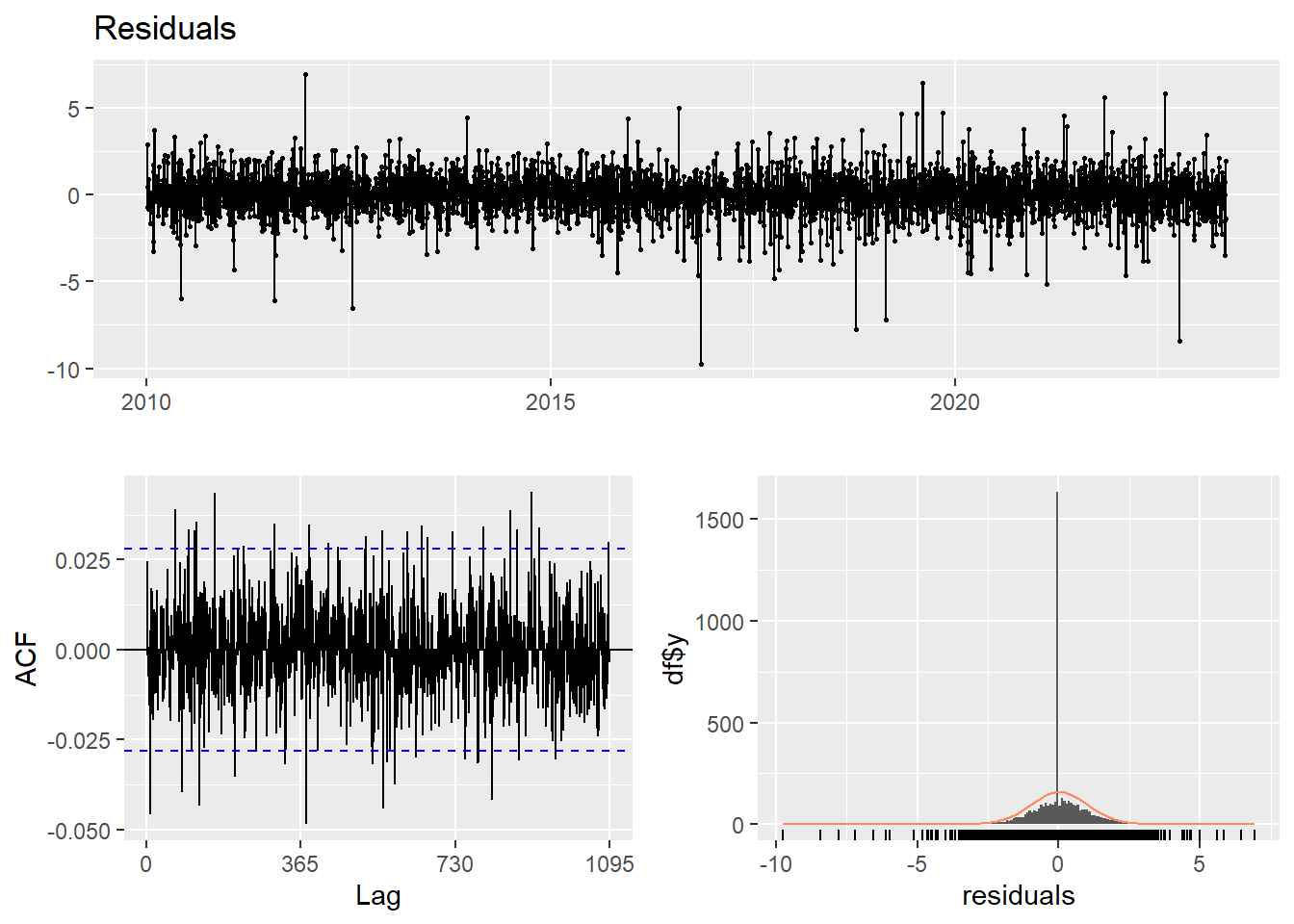
There’s still correlation left.
Volatality plot
Show the code
ht <- garch.fit1@h.t #a numeric vector with the conditional variances (h.t = sigma.t^delta)


data= data.frame(ht,CVS_df$Date[-length(CVS_df$Date)])
names(data) <- c('ht','Date')
ggplot(data, aes(y = ht, x = Date)) + geom_line(col = '#ff9933') + ylab('Conditional Variance') + xlab('Date')+ggtitle("Volatality plot")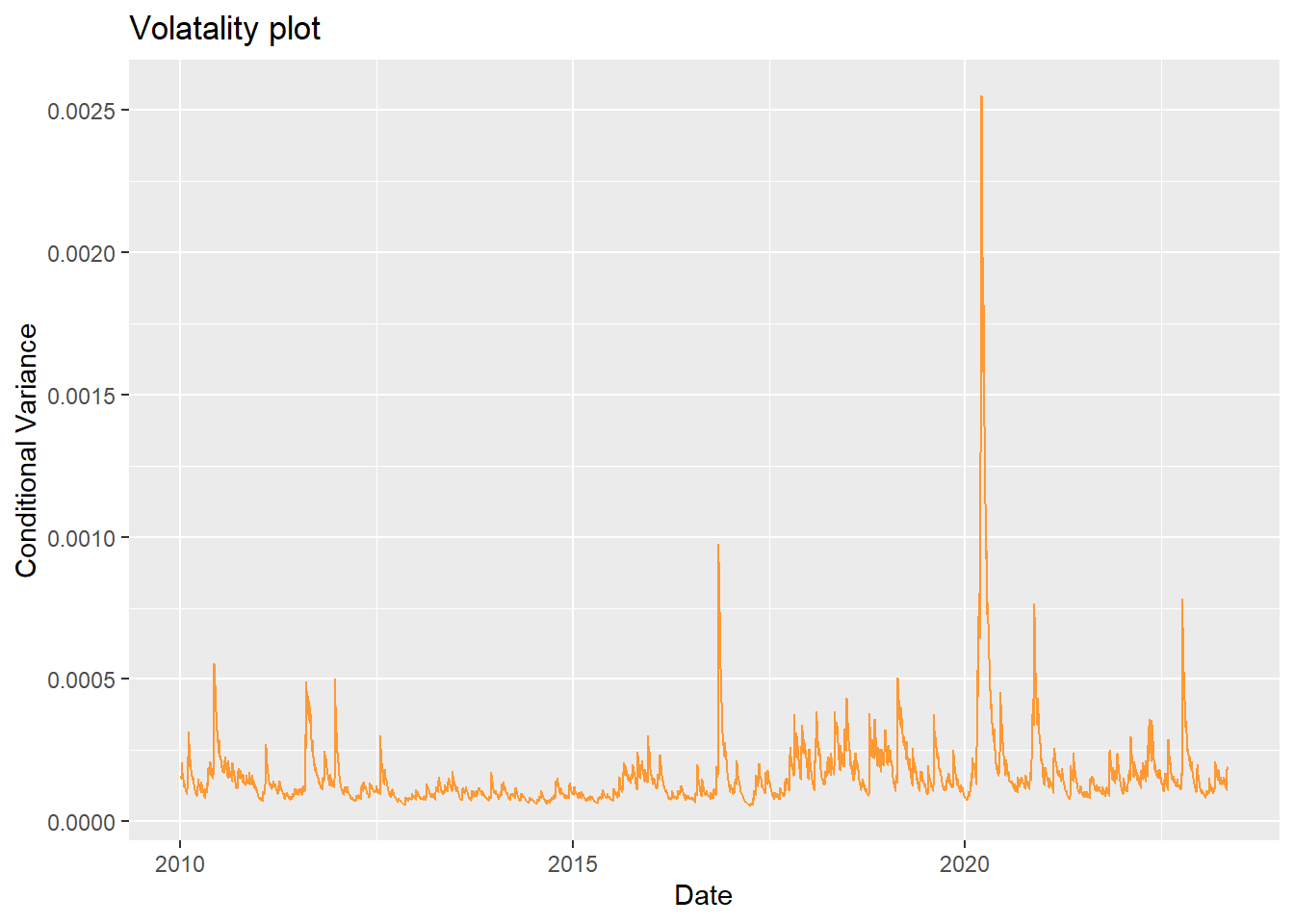
Model Comparison
We were looking at Method 1: ARIMA(0,1,0)+GARCH(1,1) and Method 2: GARCH(1,1) Perhaps Method 1 is better because Method 2 has correlation left.