ARMA/ARIMA/SARIMA Models for PFE
Step 1: Determine the stationality of time series
Stationality is a pre-requirement of training ARIMA model. This is because term ‘Auto Regressive’ in ARIMA means it is a linear regression model that uses its own lags as predictors, which work best when the predictors are not correlated and are independent of each other. Stationary time series make sure the statistical properties of time series do not change over time.
Based on information obtained from ACF graphs, the time series data is non-stationary, though Augmented Dickey-Fuller Test shows the series is stationary.
Show the code
PFE_acf <- ggAcf(PFE_ts,100)+ggtitle("PFE ACF Plot")

PFE_pacf <- ggPacf(PFE_ts)+ggtitle("PACF Plot for UHNs")
grid.arrange(PFE_acf, PFE_pacf,nrow=2)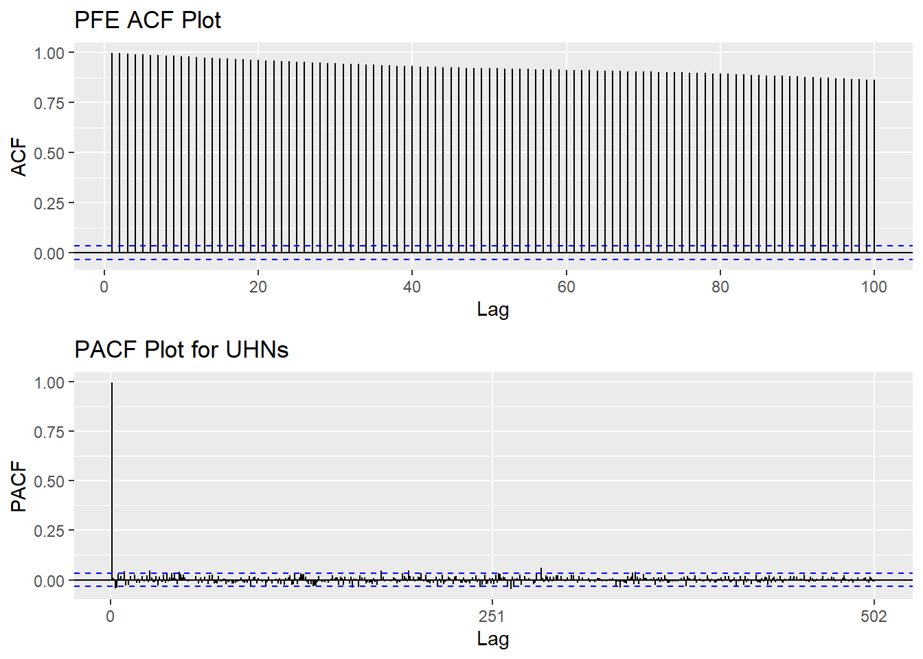
Show the code
tseries::adf.test(PFE_ts)
    Augmented Dickey-Fuller Test

data:  PFE_ts
Dickey-Fuller = -3.572, Lag order = 14, p-value = 0.03534
alternative hypothesis: stationary
Step 2: Eliminate Non-Stationality
Since this data is non-stationary, it is important to necessary to convert it to stationary time series. This step employs a series of actions to eliminate non-stationality, i.e. log transformation and differencing the data. It turns out the log transformed and 1st differened data has shown good stationary property, there are no need to go further at 2nd differencing. What is more, the Augmented Dickey-Fuller Test also confirmed that the log transformed and 1st differenced data is stationary. Therefore, the log transformation and 1st differencing would be the actions taken to eliminate the non-stationality.
Show the code
plot1<- ggAcf(log(PFE_ts) %>%diff(), 50, main="ACF Plot for Log Transformed & 1st differenced Data")
plot2<- ggAcf(log(PFE_ts) %>%diff()%>%diff(),50, main="ACF Plot for Log Transformed & 2nd differenced Data")

grid.arrange(plot1, plot2,nrow=2)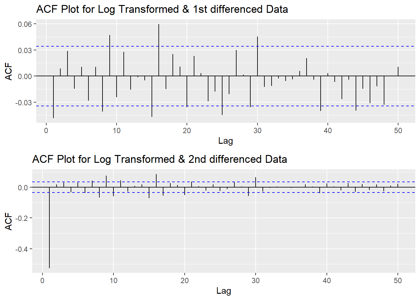
Show the code
tseries::adf.test(log(PFE_ts) %>%diff())
    Augmented Dickey-Fuller Test

data:  log(PFE_ts) %>% diff()
Dickey-Fuller = -15.533, Lag order = 14, p-value = 0.01
alternative hypothesis: stationary
Step 3: Determine p,d,q Parameters
The standard notation of ARIMA(p,d,q) include p,d,q 3 parameters. Here are the representations: - p: The number of lag observations included in the model, also called the lag order; order of the AR term. - d: The number of times that the raw observations are differenced, also called the degree of differencing; number of differencing required to make the time series stationary. - q: order of moving average; order of the MA term. It refers to the number of lagged forecast errors that should go into the ARIMA Model.
Show the code
plot3<- ggPacf(log(PFE_ts) %>%diff(),50, main="PACF Plot for Log Transformed & 1st differenced Data")

grid.arrange(plot1,plot3)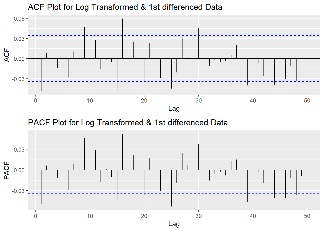
According to the PACF plot and ACF plot above, both plots have significant peak at 1. Therefore, here choose the value of both p and q as 1. Since I only differenced the data once, the d would be 1.
Step 4: Fit ARIMA(p,d,q) model
Show the code
fit1 <- Arima(log(PFE_ts), order=c(1, 1, 1),include.drift = TRUE)
summary(fit1)
Series: log(PFE_ts)
ARIMA(1,1,1) with drift
Coefficients:
ar1 ma1 drift
-0.1091 0.0608 5e-04
s.e. 0.2342 0.2348 2e-04
sigma^2 = 0.0001835: log likelihood = 9408.16
AIC=-18808.31 AICc=-18808.3 BIC=-18783.95
Training set error measures:
ME RMSE MAE MPE MAPE
Training set 3.19883e-06 0.01353642 0.009508371 -0.0009318948 0.3049848
MASE ACF1
Training set 0.05959479 -0.0001026419Model Diagnostics
- Inspection of the time plot of the standardized residuals below shows no obvious patterns.
- Notice that there may be outliers, with a few values exceeding 3 standard deviations in magnitude.
- The ACF of the standardized residuals shows no apparent departure from the model assumptions, no significant lags shown.
- The normal Q-Q plot of the residuals shows that the assumption of normality is reasonable, with the exception of the fat-tailed.
- The model appears to fit well.
Show the code
model_output <- capture.output(sarima(log(PFE_ts), 1,1,1))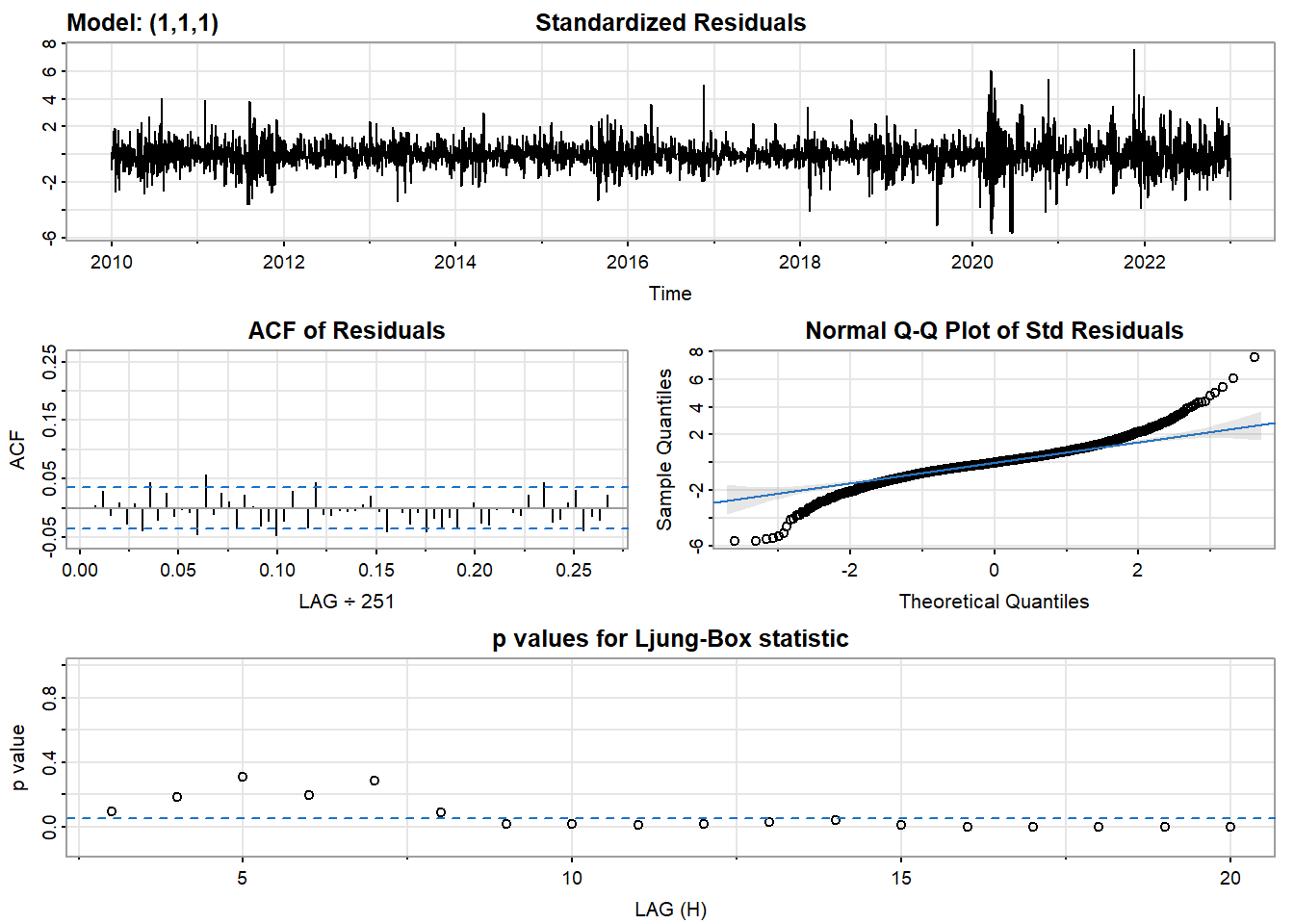
Show the code
cat(model_output[19:50], model_output[length(model_output)], sep = "\n") #to get rid of the convergence status and details of the optimization algorithm used by the sarima() $fit
Call:
arima(x = xdata, order = c(p, d, q), seasonal = list(order = c(P, D, Q), period = S),
xreg = constant, transform.pars = trans, fixed = fixed, optim.control = list(trace = trc,
REPORT = 1, reltol = tol))
Coefficients:
ar1 ma1 constant
-0.1091 0.0608 5e-04
s.e. 0.2342 0.2348 2e-04
sigma^2 estimated as 0.0001833: log likelihood = 9408.16, aic = -18808.31
$degrees_of_freedom
[1] 3260
$ttable
Estimate SE t.value p.value
ar1 -0.1091 0.2342 -0.4660 0.6412
ma1 0.0608 0.2348 0.2588 0.7958
constant 0.0005 0.0002 2.0512 0.0403
$AIC
[1] -5.764117
$AICc
[1] -5.764115
$BIC
[1] -5.756651Compare with auto.arima() function
auto.arima() returns best ARIMA model according to either AIC, AICc or BIC value. The function conducts a search over possible model within the order constraints provided. However, this method is not reliable sometimes. It fits a different model than ACF/PACF plots suggest. This is because auto.arima() usually return models that are more complex as it prefers more parameters compared than to the for example BIC.
Show the code
auto.arima(log(PFE_ts))Series: log(PFE_ts)
ARIMA(1,1,0) with drift
Coefficients:
ar1 drift
-0.0486 5e-04
s.e. 0.0175 2e-04
sigma^2 = 0.0001834: log likelihood = 9408.13
AIC=-18810.26 AICc=-18810.25 BIC=-18791.98Step 5: Forecast
The blue part in graph below forecast the next 100 values of PFE stock price in 80% and 95% confidence level.
Show the code
PFE_ts %>%
  Arima(order=c(1,1,1),include.drift = TRUE) %>%
  forecast(100) %>%
  autoplot() +
  ylab("PFE stock prices prediction") + xlab("Year")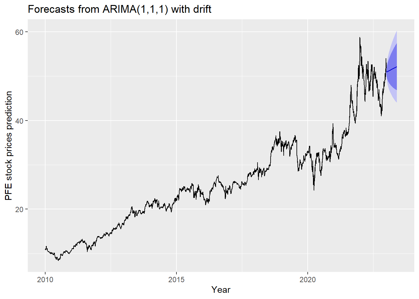
Step 6: Compare ARIMA model with the benchmark methods
Forecasting benchmarks are very important when testing new forecasting methods, to see how well they perform against some simple alternatives.
Average method
Here, the forecast of all future values are equal to the average of the historical data. The residual plot of this method is not stationary.
Show the code
f1<-meanf(log(PFE_ts), h=251) #mean
#summary(f1)
checkresiduals(f1)#serial correlation ; Lung Box p <0.05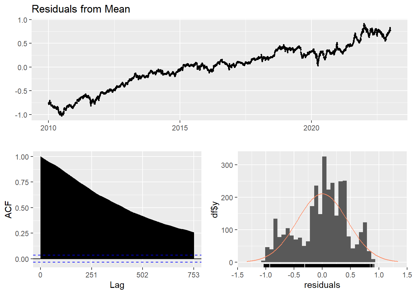
    Ljung-Box test

data:  Residuals from Mean
Q* = 869974, df = 501, p-value < 2.2e-16

Model df: 1.   Total lags used: 502
Naive method
This method simply set all forecasts to be the value of the last observation. According to error measurement here, ARIMA(1,1,1) outperform the average method.
Show the code
f2<-naive(log(PFE_ts), h=11) # naive method
summary(f2)
Forecast method: Naive method

Model Information:
Call: naive(y = log(PFE_ts), h = 11)

Residual sd: 0.0136

Error measures:
                       ME       RMSE         MAE        MPE      MAPE
Training set 0.0004687069 0.01356269 0.009523496 0.01416351 0.3054974
                   MASE        ACF1
Training set 0.05968959 -0.04862067

Forecasts:
         Point Forecast    Lo 80    Hi 80    Lo 95    Hi 95
2023.004       3.929721 3.912340 3.947102 3.903139 3.956303
2023.008       3.929721 3.905140 3.954302 3.892128 3.967314
2023.012       3.929721 3.899616 3.959826 3.883679 3.975763
2023.016       3.929721 3.894959 3.964484 3.876556 3.982886
2023.020       3.929721 3.890855 3.968587 3.870281 3.989161
2023.024       3.929721 3.887146 3.972296 3.864608 3.994834
2023.028       3.929721 3.883735 3.975708 3.859391 4.000051
2023.032       3.929721 3.880559 3.978883 3.854535 4.004907
2023.036       3.929721 3.877577 3.981865 3.849974 4.009468
2023.040       3.929721 3.874757 3.984686 3.845660 4.013782
2023.044       3.929721 3.872074 3.987368 3.841557 4.017885
Show the code
checkresiduals(f2)#serial correlation ; Lung Box p <0.05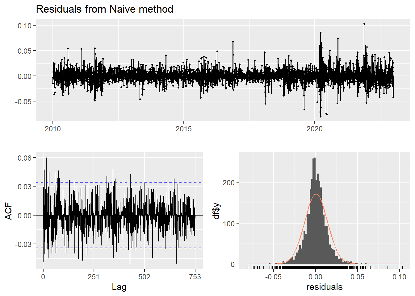
    Ljung-Box test

data:  Residuals from Naive method
Q* = 599.92, df = 502, p-value = 0.001694

Model df: 0.   Total lags used: 502
Seasonal naive method
This method is useful for highly seasonal data, which can set each forecast to be equal to the last observed value from the same season of the year. Here seasonal naive is used to forecast the next 4 values for the PFE stock price series.
Show the code
f3<-snaive(log(PFE_ts), h=4) #seasonal naive method
summary(f3)
Forecast method: Seasonal naive method

Model Information:
Call: snaive(y = log(PFE_ts), h = 4)

Residual sd: 0.1904

Error measures:
                    ME      RMSE       MAE      MPE   MAPE MASE      ACF1
Training set 0.1322592 0.1903849 0.1595504 4.188333 5.0082    1 0.9895735

Forecasts:
         Point Forecast    Lo 80    Hi 80    Lo 95    Hi 95
2023.004       4.035591 3.791603 4.279579 3.662443 4.408738
2023.008       4.045718 3.801730 4.289706 3.672570 4.418865
2023.012       4.031511 3.787523 4.275499 3.658364 4.404659
2023.016       4.039823 3.795835 4.283811 3.666675 4.412970
Show the code
checkresiduals(f3) #serial correlation ; Lung Box p <0.05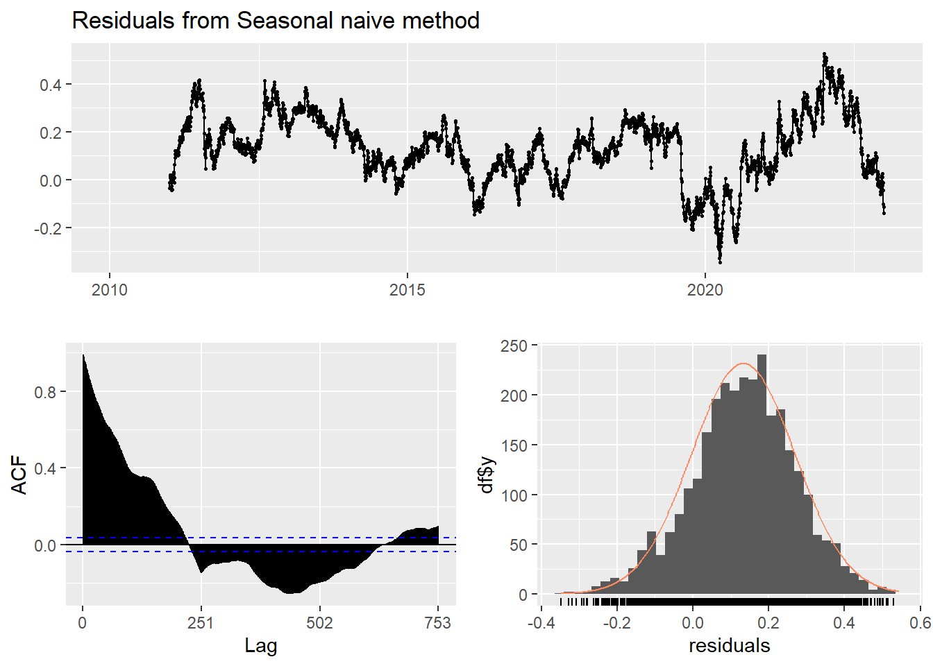
    Ljung-Box test

data:  Residuals from Seasonal naive method
Q* = 194683, df = 502, p-value < 2.2e-16

Model df: 0.   Total lags used: 502
Drift Method
A variation on the naïve method is to allow the forecasts to increase or decrease over time, where the amount of change over time is set to be the average change seen in the historical data.
Show the code
f4 <- rwf(log(PFE_ts),drift=TRUE, h=20)
summary(f4)
Forecast method: Random walk with drift

Model Information:
Call: rwf(y = log(PFE_ts), h = 20, drift = TRUE)

Drift: 5e-04  (se 2e-04)
Residual sd: 0.0136

Error measures:
                        ME       RMSE        MAE          MPE      MAPE
Training set -1.352823e-16 0.01355458 0.00952708 -0.001001816 0.3056554
                   MASE        ACF1
Training set 0.05971205 -0.04862067

Forecasts:
         Point Forecast    Lo 80    Hi 80    Lo 95    Hi 95
2023.004       3.930190 3.912814 3.947566 3.903615 3.956764
2023.008       3.930658 3.906081 3.955236 3.893071 3.968246
2023.012       3.931127 3.901021 3.961233 3.885084 3.977170
2023.016       3.931596 3.896827 3.966364 3.878422 3.984770
2023.020       3.932065 3.893186 3.970943 3.872606 3.991524
2023.024       3.932533 3.889938 3.975129 3.867389 3.997677
2023.028       3.933002 3.886987 3.979017 3.862628 4.003376
2023.032       3.933471 3.884271 3.982671 3.858226 4.008716
2023.036       3.933939 3.881747 3.986132 3.854118 4.013761
2023.040       3.934408 3.879384 3.989432 3.850256 4.018560
2023.044       3.934877 3.877158 3.992595 3.846604 4.023150
2023.048       3.935346 3.875051 3.995640 3.843133 4.027558
2023.052       3.935814 3.873048 3.998580 3.839822 4.031806
2023.056       3.936283 3.871138 4.001428 3.836652 4.035914
2023.060       3.936752 3.869310 4.004194 3.833608 4.039895
2023.064       3.937220 3.867556 4.006885 3.830678 4.043763
2023.068       3.937689 3.865870 4.009508 3.827851 4.047527
2023.072       3.938158 3.864245 4.012071 3.825118 4.051198
2023.076       3.938626 3.862677 4.014576 3.822471 4.054782
2023.080       3.939095 3.861161 4.017030 3.819904 4.058286
Show the code
checkresiduals(f4)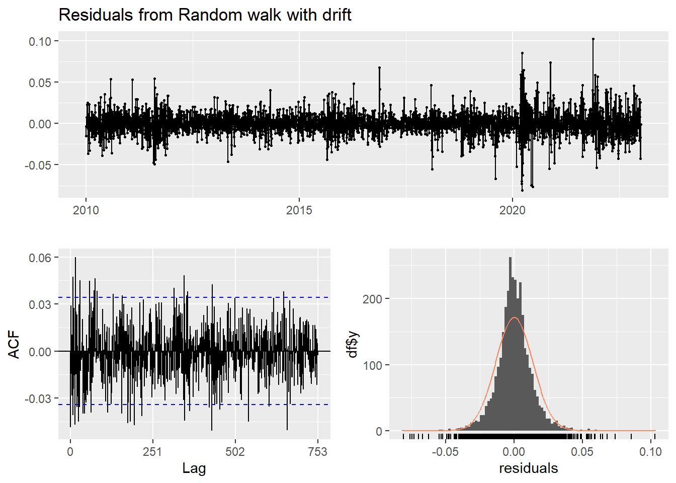
    Ljung-Box test

data:  Residuals from Random walk with drift
Q* = 599.92, df = 501, p-value = 0.001534

Model df: 1.   Total lags used: 502
Show the code
autoplot(PFE_ts) +
  autolayer(meanf(PFE_ts, h=100),
            series="Mean.tr", PI=FALSE) +
  autolayer(naive((PFE_ts), h=100),
            series="Naïve.tr", PI=FALSE) +
  autolayer(rwf((PFE_ts), drift=TRUE, h=100),
            series="Drift.tr", PI=FALSE) +
  autolayer(forecast(Arima((PFE_ts), order=c(1, 1, 1),include.drift = TRUE),100),
            series="fit",PI=FALSE) +
  ggtitle("PFE Stock Price") +
  xlab("Time") + ylab("Log(Price)") +
  guides(colour=guide_legend(title="Forecast"))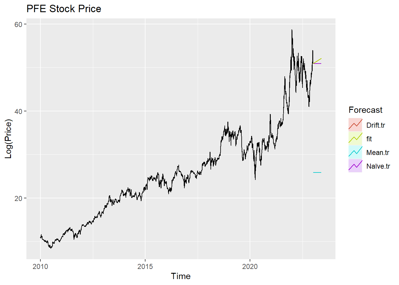
According to the graph above, ARIMA(1,1,1) outperform most of benchmark method, though its performance is very similar to drift method.