ARMA/ARIMA/SARIMA Models for AZN
Step 1: Determine the stationality of time series
Stationality is a pre-requirement of training ARIMA model. This is because term ‘Auto Regressive’ in ARIMA means it is a linear regression model that uses its own lags as predictors, which work best when the predictors are not correlated and are independent of each other. Stationary time series make sure the statistical properties of time series do not change over time.
Based on information obtained from both ACF graphs and Augmented Dickey-Fuller Test, the time series data is non-stationary.
Show the code
AZN_acf <- ggAcf(AZN_ts,100)+ggtitle("AZN ACF Plot")

AZN_pacf <- ggPacf(AZN_ts)+ggtitle("PACF Plot for UHNs")
grid.arrange(AZN_acf, AZN_pacf,nrow=2)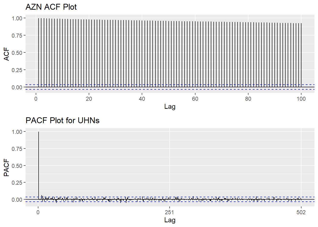
Show the code
tseries::adf.test(AZN_ts)
    Augmented Dickey-Fuller Test

data:  AZN_ts
Dickey-Fuller = -3.3602, Lag order = 14, p-value = 0.06026
alternative hypothesis: stationary
Step 2: Eliminate Non-Stationality
Since this data is non-stationary, it is important to necessary to convert it to stationary time series. This step employs a series of actions to eliminate non-stationality, i.e. log transformation and differencing the data. It turns out the log transformed and 1st differened data has shown good stationary property, there are no need to go further at 2nd differencing. What is more, the Augmented Dickey-Fuller Test also confirmed that the log transformed and 1st differenced data is stationary. Therefore, the log transformation and 1st differencing would be the actions taken to eliminate the non-stationality.
Show the code
plot1<- ggAcf(log(AZN_ts) %>%diff(), 50, main="ACF Plot for Log Transformed & 1st differenced Data")
plot2<- ggAcf(log(AZN_ts) %>%diff()%>%diff(),50, main="ACF Plot for Log Transformed & 2nd differenced Data")

grid.arrange(plot1, plot2,nrow=2)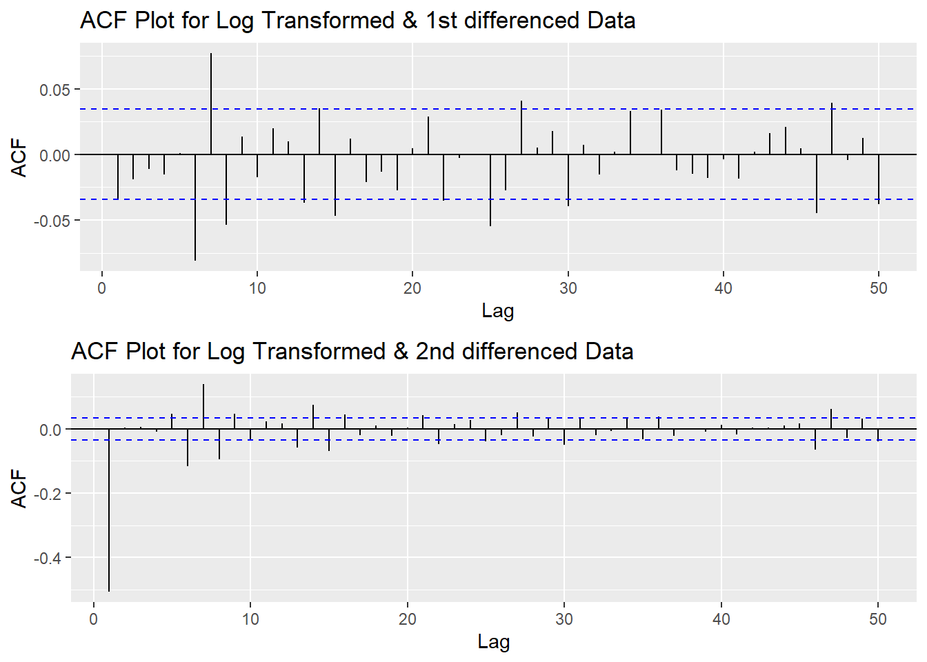
Show the code
tseries::adf.test(log(AZN_ts) %>%diff())
    Augmented Dickey-Fuller Test

data:  log(AZN_ts) %>% diff()
Dickey-Fuller = -15.655, Lag order = 14, p-value = 0.01
alternative hypothesis: stationary
Step 3: Determine p,d,q Parameters
The standard notation of ARIMA(p,d,q) include p,d,q 3 parameters. Here are the representations: - p: The number of lag observations included in the model, also called the lag order; order of the AR term. - d: The number of times that the raw observations are differenced, also called the degree of differencing; number of differencing required to make the time series stationary. - q: order of moving average; order of the MA term. It refers to the number of lagged forecast errors that should go into the ARIMA Model.
Show the code
plot3<- ggPacf(log(AZN_ts) %>%diff(),50, main="PACF Plot for Log Transformed & 1st differenced Data")

grid.arrange(plot1,plot3)
According to the PACF plot and ACF plot above, both plots have 3 significant peak at 6,7,8. To avoid over-complexity, here choose the value of p and q as 0. Since I only differenced the data once, the d would be 1.
Step 4: Fit ARIMA(p,d,q) model
Show the code
fit1 <- Arima(log(AZN_ts), order=c(0, 1, 0),include.drift = TRUE)
summary(fit1)
Series: log(AZN_ts)
ARIMA(0,1,0) with drift
Coefficients:
drift
5e-04
s.e. 3e-04
sigma^2 = 0.0002423: log likelihood = 8953.58
AIC=-17903.16 AICc=-17903.16 BIC=-17890.98
Training set error measures:
ME RMSE MAE MPE MAPE
Training set 1.15802e-06 0.01555995 0.01046885 -0.0005720625 0.227243
MASE ACF1
Training set 0.05903222 -0.03420903Model Diagnostics
- Inspection of the time plot of the standardized residuals below shows no obvious patterns.
- Notice that there may be outliers, with a few values exceeding 3 standard deviations in magnitude.
- The ACF of the standardized residuals shows no apparent departure from the model assumptions, no significant lags shown.
- The normal Q-Q plot of the residuals shows that the assumption of normality is reasonable, with the exception of the fat-tailed.
- The model appears to fit well.
Show the code
model_output <- capture.output(sarima(log(AZN_ts), 0,1,0))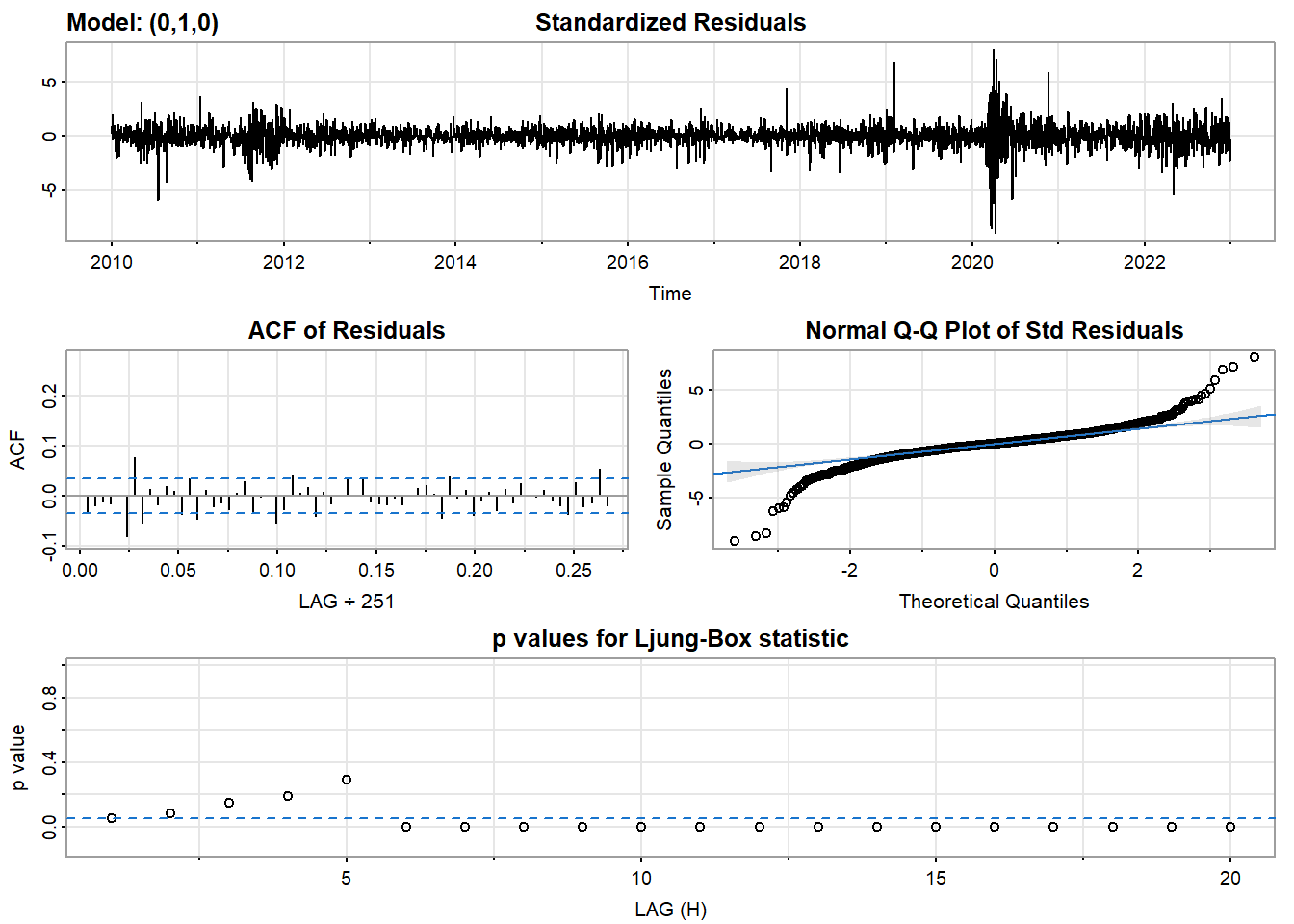
Show the code
cat(model_output[9:38], model_output[length(model_output)], sep = "\n") #to get rid of the convergence status and details of the optimization algorithm used by the sarima() $fit
Call:
arima(x = xdata, order = c(p, d, q), seasonal = list(order = c(P, D, Q), period = S),
xreg = constant, transform.pars = trans, fixed = fixed, optim.control = list(trace = trc,
REPORT = 1, reltol = tol))
Coefficients:
constant
5e-04
s.e. 3e-04
sigma^2 estimated as 0.0002422: log likelihood = 8953.58, aic = -17903.16
$degrees_of_freedom
[1] 3262
$ttable
Estimate SE t.value p.value
constant 5e-04 3e-04 1.8978 0.0578
$AIC
[1] -5.486718
$AICc
[1] -5.486718
$BIC
[1] -5.482985Compare with auto.arima() function
auto.arima() returns best ARIMA model according to either AIC, AICc or BIC value. The function conducts a search over possible model within the order constraints provided. However, this method is not reliable sometimes. It fits a different model than ACF/PACF plots suggest. This is because auto.arima() usually return models that are more complex as it prefers more parameters compared than to the for example BIC.
Show the code
auto.arima(log(AZN_ts))Series: log(AZN_ts)
ARIMA(1,1,1) with drift
Coefficients:
ar1 ma1 drift
0.9292 -0.9519 5e-04
s.e. 0.0365 0.0305 2e-04
sigma^2 = 0.0002415: log likelihood = 8959.68
AIC=-17911.36 AICc=-17911.35 BIC=-17887Step 5: Forecast
The blue part in graph below forecast the next 100 values of AZN stock price in 80% and 95% confidence level.
Show the code
log(AZN_ts) %>%
  Arima(order=c(0,1,0),include.drift = TRUE) %>%
  forecast(100) %>%
  autoplot() +
  ylab("AZN stock prices prediction") + xlab("Year")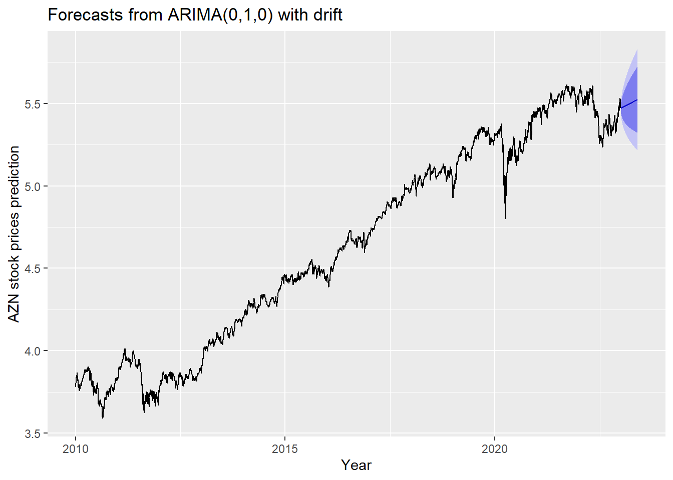
Step 6: Compare ARIMA model with the benchmark methods
Forecasting benchmarks are very important when testing new forecasting methods, to see how well they perform against some simple alternatives.
Average method
Here, the forecast of all future values are equal to the average of the historical data. The residual plot of this method is not stationary.
Show the code
f1<-meanf(log(AZN_ts), h=251) #mean
#summary(f1)
checkresiduals(f1)#serial correlation ; Lung Box p <0.05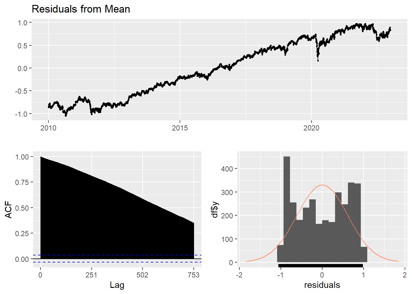
    Ljung-Box test

data:  Residuals from Mean
Q* = 1165071, df = 501, p-value < 2.2e-16

Model df: 1.   Total lags used: 502
Naive method
This method simply set all forecasts to be the value of the last observation. According to error measurement here, ARIMA(0,1,0) outperform the average method.
Show the code
f2<-naive(log(AZN_ts), h=11) # naive method
summary(f2)
Forecast method: Naive method

Model Information:
Call: naive(y = log(AZN_ts), h = 11)

Residual sd: 0.0156

Error measures:
                       ME       RMSE        MAE        MPE      MAPE       MASE
Training set 0.0005180792 0.01557082 0.01049512 0.01076463 0.2277994 0.05918031
                    ACF1
Training set -0.03425189

Forecasts:
         Point Forecast    Lo 80    Hi 80    Lo 95    Hi 95
2023.004       5.470789 5.450834 5.490744 5.440271 5.501307
2023.008       5.470789 5.442569 5.499010 5.427630 5.513949
2023.012       5.470789 5.436226 5.505352 5.417930 5.523648
2023.016       5.470789 5.430880 5.510699 5.409753 5.531826
2023.020       5.470789 5.426169 5.515410 5.402548 5.539030
2023.024       5.470789 5.421910 5.519668 5.396035 5.545543
2023.028       5.470789 5.417994 5.523585 5.390046 5.551533
2023.032       5.470789 5.414349 5.527230 5.384471 5.557108
2023.036       5.470789 5.410925 5.530654 5.379234 5.562344
2023.040       5.470789 5.407687 5.533892 5.374282 5.567296
2023.044       5.470789 5.404607 5.536972 5.369572 5.572007
Show the code
checkresiduals(f2)#serial correlation ; Lung Box p <0.05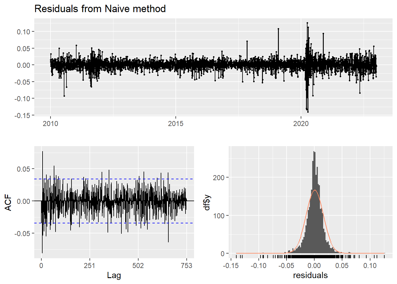
    Ljung-Box test

data:  Residuals from Naive method
Q* = 627.23, df = 502, p-value = 0.0001143

Model df: 0.   Total lags used: 502
Seasonal naive method
This method is useful for highly seasonal data, which can set each forecast to be equal to the last observed value from the same season of the year. Here seasonal naive is used to forecast the next 4 values for the AZN stock price series.
Show the code
f3<-snaive(log(AZN_ts), h=4) #seasonal naive method
summary(f3)
Forecast method: Seasonal naive method

Model Information:
Call: snaive(y = log(AZN_ts), h = 4)

Residual sd: 0.1989

Error measures:
                    ME      RMSE       MAE      MPE     MAPE MASE      ACF1
Training set 0.1378916 0.1988982 0.1773414 2.933481 3.770862    1 0.9881511

Forecasts:
         Point Forecast    Lo 80    Hi 80    Lo 95    Hi 95
2023.004       5.528218 5.273320 5.783116 5.138385 5.918052
2023.008       5.558320 5.303422 5.813219 5.168487 5.948154
2023.012       5.574101 5.319203 5.828999 5.184268 5.963934
2023.016       5.582158 5.327260 5.837056 5.192325 5.971991
Show the code
checkresiduals(f3) #serial correlation ; Lung Box p <0.05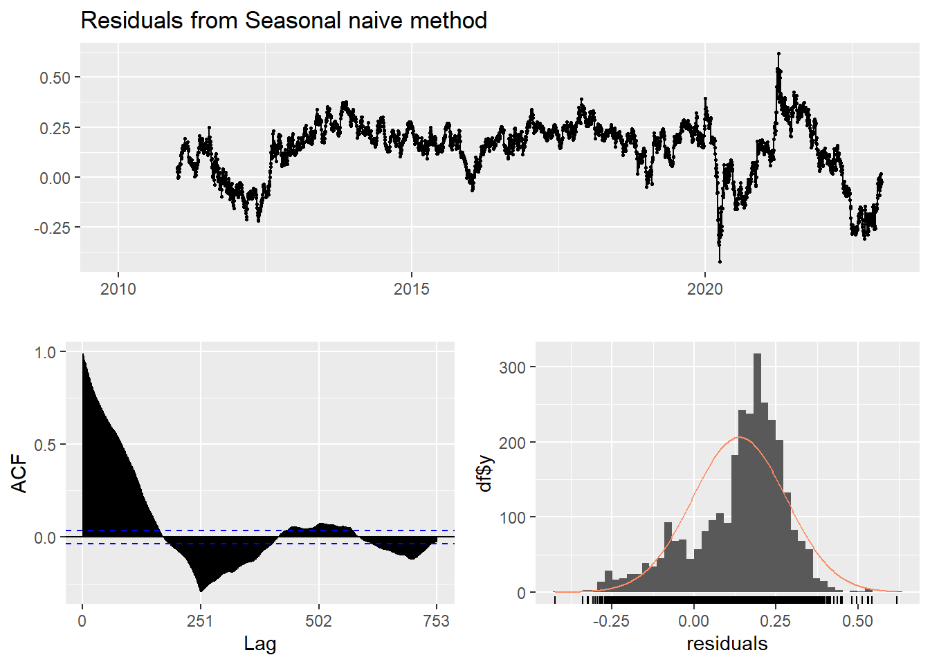
    Ljung-Box test

data:  Residuals from Seasonal naive method
Q* = 174670, df = 502, p-value < 2.2e-16

Model df: 0.   Total lags used: 502
Drift Method
A variation on the naïve method is to allow the forecasts to increase or decrease over time, where the amount of change over time is set to be the average change seen in the historical data.
Show the code
f4 <- rwf(log(AZN_ts),drift=TRUE, h=20)
summary(f4)
Forecast method: Random walk with drift

Model Information:
Call: rwf(y = log(AZN_ts), h = 20, drift = TRUE)

Drift: 5e-04  (se 3e-04)
Residual sd: 0.0156

Error measures:
                       ME      RMSE       MAE           MPE     MAPE       MASE
Training set 2.353136e-16 0.0155622 0.0104709 -0.0006028803 0.227282 0.05904378
                    ACF1
Training set -0.03425189

Forecasts:
         Point Forecast    Lo 80    Hi 80    Lo 95    Hi 95
2023.004       5.471307 5.451357 5.491257 5.440797 5.501818
2023.008       5.471825 5.443608 5.500043 5.428670 5.514981
2023.012       5.472343 5.437779 5.506908 5.419481 5.525206
2023.016       5.472862 5.432943 5.512780 5.411812 5.533911
2023.020       5.473380 5.428743 5.518016 5.405114 5.541645
2023.024       5.473898 5.424993 5.522802 5.399105 5.548691
2023.028       5.474416 5.421585 5.527247 5.393618 5.555214
2023.032       5.474934 5.418447 5.531421 5.388544 5.561324
2023.036       5.475452 5.415529 5.535375 5.383808 5.567096
2023.040       5.475970 5.412796 5.539144 5.379354 5.572586
2023.044       5.476488 5.410221 5.542756 5.375141 5.577836
2023.048       5.477006 5.407781 5.546231 5.371136 5.582876
2023.052       5.477524 5.405462 5.549587 5.367314 5.587734
2023.056       5.478042 5.403248 5.552836 5.363655 5.592430
2023.060       5.478560 5.401129 5.555991 5.360140 5.596981
2023.064       5.479078 5.399096 5.559061 5.356756 5.601401
2023.068       5.479597 5.397140 5.562053 5.353490 5.605703
2023.072       5.480115 5.395254 5.564975 5.350332 5.609897
2023.076       5.480633 5.393434 5.567832 5.347273 5.613992
2023.080       5.481151 5.391673 5.570629 5.344306 5.617995
Show the code
checkresiduals(f4)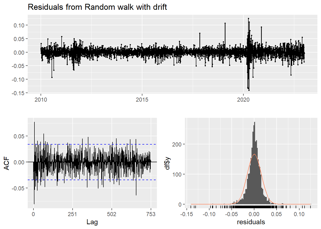
    Ljung-Box test

data:  Residuals from Random walk with drift
Q* = 627.23, df = 501, p-value = 0.0001014

Model df: 1.   Total lags used: 502
Show the code
autoplot(AZN_ts) +
  autolayer(meanf(AZN_ts, h=100),
            series="Mean.tr", PI=FALSE) +
  autolayer(naive((AZN_ts), h=100),
            series="Naïve.tr", PI=FALSE) +
  autolayer(rwf((AZN_ts), drift=TRUE, h=100),
            series="Drift.tr", PI=FALSE) +
  autolayer(forecast(Arima((AZN_ts), order=c(4, 1, 3),include.drift = TRUE),100),
            series="fit",PI=FALSE) +
  ggtitle("AZN Stock Price") +
  xlab("Time") + ylab("Log(Price)") +
  guides(colour=guide_legend(title="Forecast"))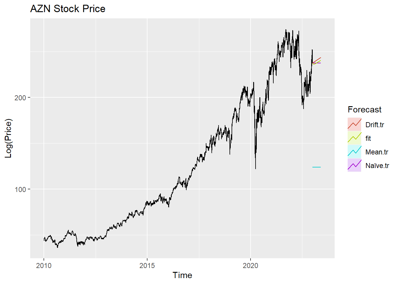
According to the graph above, ARIMA(0,1,0) outperform most of benchmark method, though its performance is very similar to drift method.