GPD
EDA
Show the code
gdp <- read.csv('data/Employment59.csv')
gdp$DATE <- as.Date(gdp$DATE)
gdp_ts <- ts(gdp$PAYEMS, star= c(1959,1),frequency = 4)
autoplot(gdp_ts)+ggtitle("US GDP")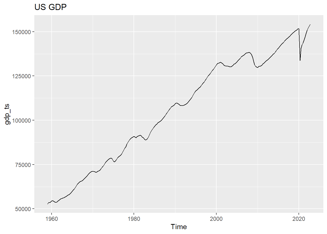
Show the code
acf(gdp_ts)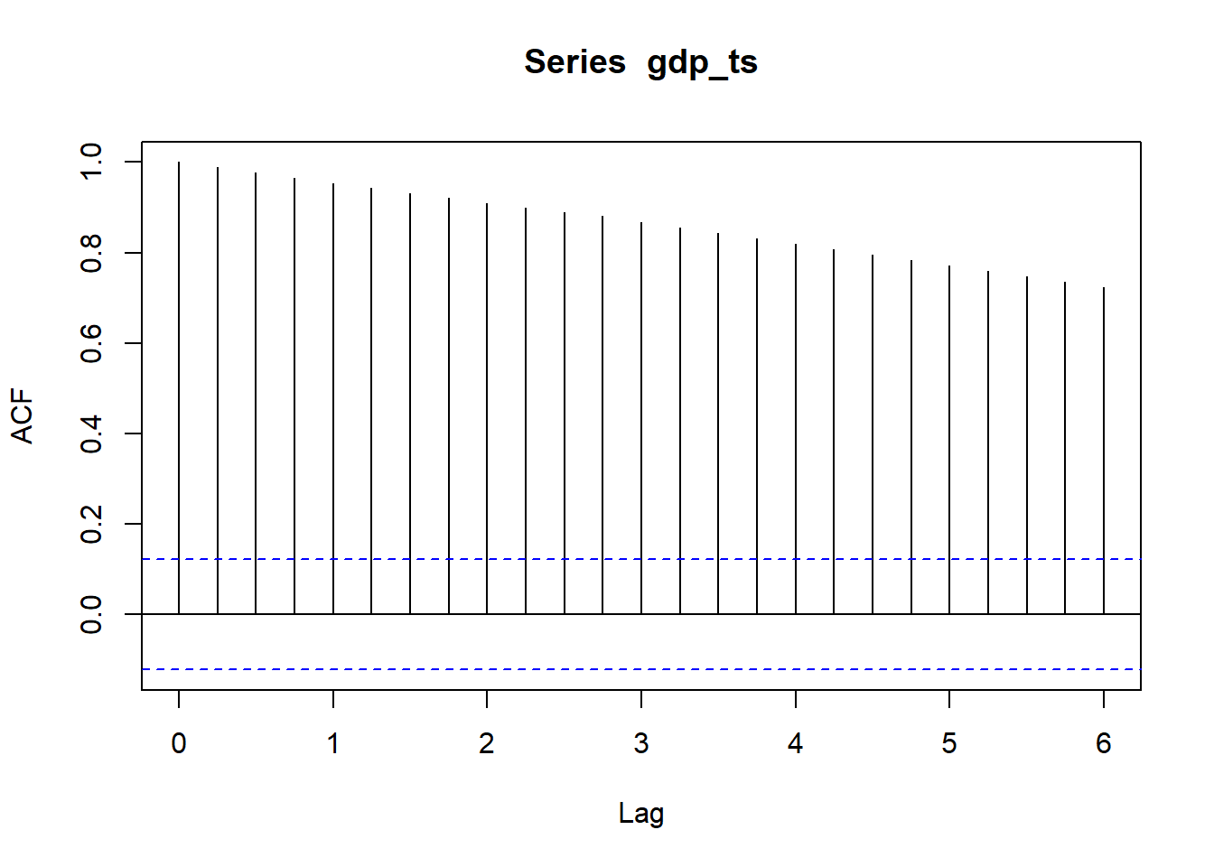
Show the code
dec2=decompose(gdp_ts,type = "multiplicative")
plot(dec2)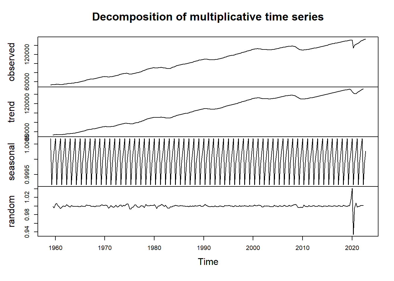
Show the code
gdp_ts %>% diff() %>% ggtsdisplay() #first ordinary differencing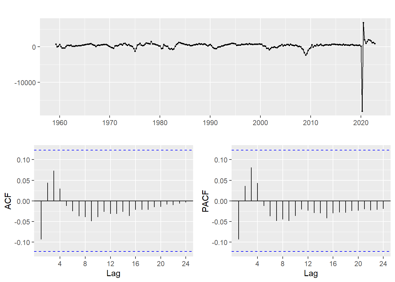
Show the code
gdp_ts %>% diff(lag = 4) %>% ggtsdisplay() #first ordinary differencing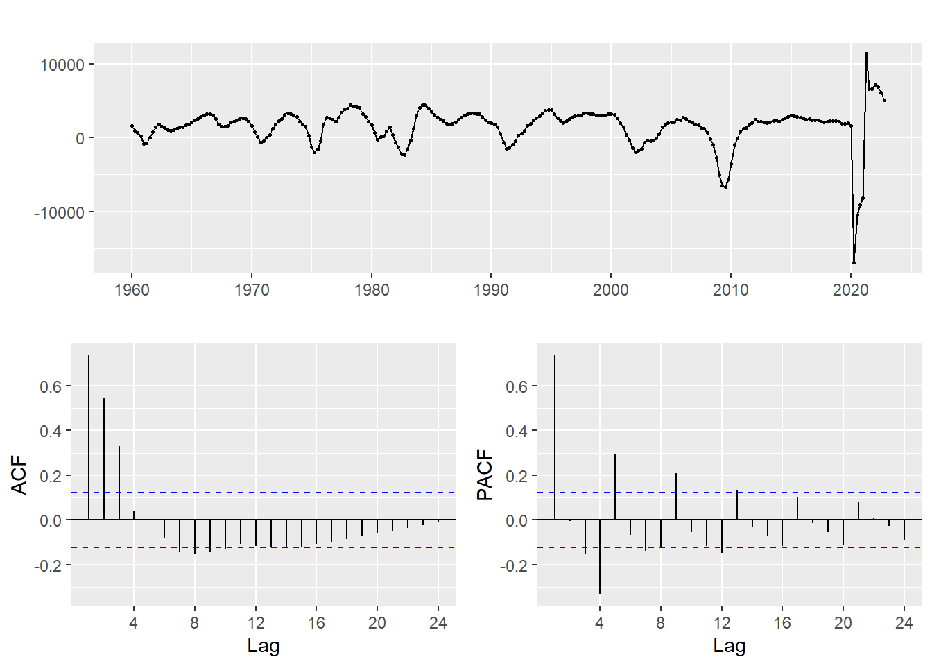
Determine Parameters
Show the code
gdp_ts %>% diff(lag=4) %>% diff() %>% ggtsdisplay() #do both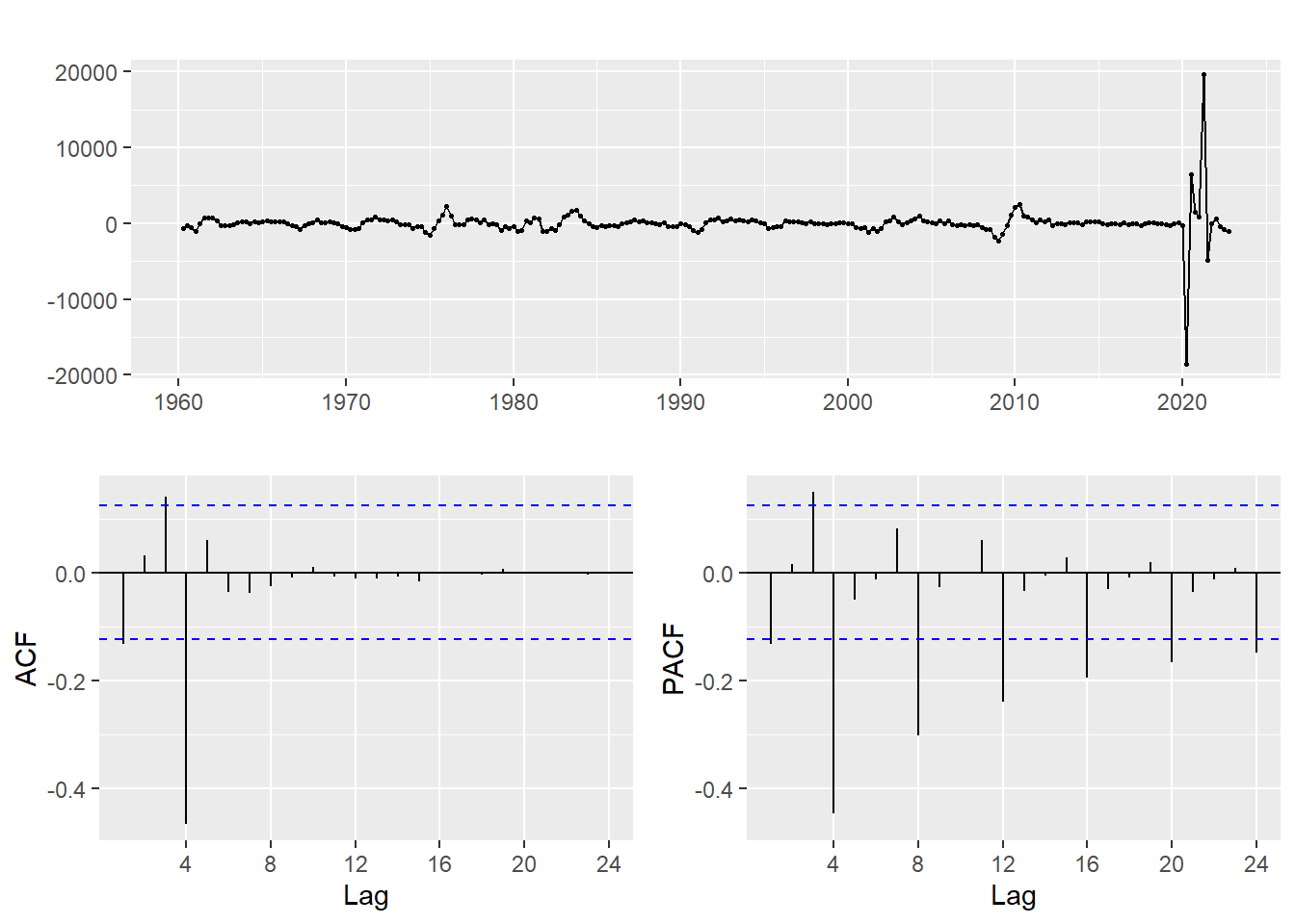
p:0,1,3 d:2 q:1,2,3 P:1,2,3 D:2 Q:1
Show the code
######################## Check for different combinations ########


#write a funtion
SARIMA.c=function(p1,p2,q1,q2,P1,P2,Q1,Q2,data){

  #K=(p2+1)*(q2+1)*(P2+1)*(Q2+1)

  temp=c()
  d=1
  D=1
  s=12

  i=1
  temp= data.frame()
  ls=matrix(rep(NA,9*35),nrow=35)


  for (p in p1:p2)
  {
    for(q in q1:q2)
    {
      for(P in P1:P2)
      {
        for(Q in Q1:Q2)
        {
          if(p+d+q+P+D+Q<=9)
          {

            model<- Arima(data,order=c(p-1,d,q-1),seasonal=c(P-1,D,Q-1))
            ls[i,]= c(p-1,d,q-1,P-1,D,Q-1,model$aic,model$bic,model$aicc)
            i=i+1
            #print(i)

          }

        }
      }
    }

  }


  temp= as.data.frame(ls)
  names(temp)= c("p","d","q","P","D","Q","AIC","BIC","AICc")

  temp

}

output = SARIMA.c(p1=1,p2=4,q1=1,q2=4,P1=1,P2=3,Q1=1,Q2=2, data = gdp_ts)
#output

knitr::kable(output)| p | d | q | P | D | Q | AIC | BIC | AICc |
|---|---|---|---|---|---|---|---|---|
| 0 | 1 | 0 | 0 | 1 | 0 | 4498.257 | 4501.782 | 4498.273 |
| 0 | 1 | 0 | 0 | 1 | 1 | 4348.055 | 4355.106 | 4348.104 |
| 0 | 1 | 0 | 1 | 1 | 0 | 4439.336 | 4446.387 | 4439.384 |
| 0 | 1 | 0 | 1 | 1 | 1 | 4350.031 | 4360.607 | 4350.128 |
| 0 | 1 | 0 | 2 | 1 | 0 | 4379.073 | 4389.649 | 4379.170 |
| 0 | 1 | 0 | 2 | 1 | 1 | 4350.737 | 4364.839 | 4350.900 |
| 0 | 1 | 1 | 0 | 1 | 0 | 4496.142 | 4503.193 | 4496.191 |
| 0 | 1 | 1 | 0 | 1 | 1 | 4348.392 | 4358.968 | 4348.489 |
| 0 | 1 | 1 | 1 | 1 | 0 | 4439.612 | 4450.188 | 4439.709 |
| 0 | 1 | 1 | 1 | 1 | 1 | 4350.294 | 4364.396 | 4350.456 |
| 0 | 1 | 1 | 2 | 1 | 0 | 4381.060 | 4395.162 | 4381.223 |
| 0 | 1 | 2 | 0 | 1 | 0 | 4488.150 | 4498.727 | 4488.248 |
| 0 | 1 | 2 | 0 | 1 | 1 | 4349.256 | 4363.357 | 4349.418 |
| 0 | 1 | 2 | 1 | 1 | 0 | 4440.078 | 4454.180 | 4440.241 |
| 0 | 1 | 3 | 0 | 1 | 0 | 4478.378 | 4492.480 | 4478.541 |
| 1 | 1 | 0 | 0 | 1 | 0 | 4495.859 | 4502.910 | 4495.907 |
| 1 | 1 | 0 | 0 | 1 | 1 | 4348.206 | 4358.782 | 4348.303 |
| 1 | 1 | 0 | 1 | 1 | 0 | 4439.428 | 4450.005 | 4439.525 |
| 1 | 1 | 0 | 1 | 1 | 1 | 4350.101 | 4364.203 | 4350.264 |
| 1 | 1 | 0 | 2 | 1 | 0 | 4381.057 | 4395.159 | 4381.220 |
| 1 | 1 | 1 | 0 | 1 | 0 | 4497.843 | 4508.419 | 4497.940 |
| 1 | 1 | 1 | 0 | 1 | 1 | 4350.038 | 4364.139 | 4350.200 |
| 1 | 1 | 1 | 1 | 1 | 0 | 4441.326 | 4455.428 | 4441.489 |
| 1 | 1 | 2 | 0 | 1 | 0 | 4489.217 | 4503.319 | 4489.380 |
| 2 | 1 | 0 | 0 | 1 | 0 | 4497.803 | 4508.379 | 4497.900 |
| 2 | 1 | 0 | 0 | 1 | 1 | 4349.683 | 4363.785 | 4349.845 |
| 2 | 1 | 0 | 1 | 1 | 0 | 4441.003 | 4455.105 | 4441.165 |
| 2 | 1 | 1 | 0 | 1 | 0 | 4499.678 | 4513.780 | 4499.841 |
| 3 | 1 | 0 | 0 | 1 | 0 | 4494.238 | 4508.340 | 4494.400 |
| NA | NA | NA | NA | NA | NA | NA | NA | NA |
| NA | NA | NA | NA | NA | NA | NA | NA | NA |
| NA | NA | NA | NA | NA | NA | NA | NA | NA |
| NA | NA | NA | NA | NA | NA | NA | NA | NA |
| NA | NA | NA | NA | NA | NA | NA | NA | NA |
| NA | NA | NA | NA | NA | NA | NA | NA | NA |
Show the code
output[which.min(output$AIC),] p d q P D Q AIC BIC AICc
2 0 1 0 0 1 1 4348.055 4355.106 4348.104Show the code
output[which.min(output$BIC),] p d q P D Q AIC BIC AICc
2 0 1 0 0 1 1 4348.055 4355.106 4348.104Show the code
output[which.min(output$AICc),] p d q P D Q AIC BIC AICc
2 0 1 0 0 1 1 4348.055 4355.106 4348.104Show the code
set.seed(123)
model_output <- capture.output(sarima(gdp_ts, 0,1,0,0,1,1,4))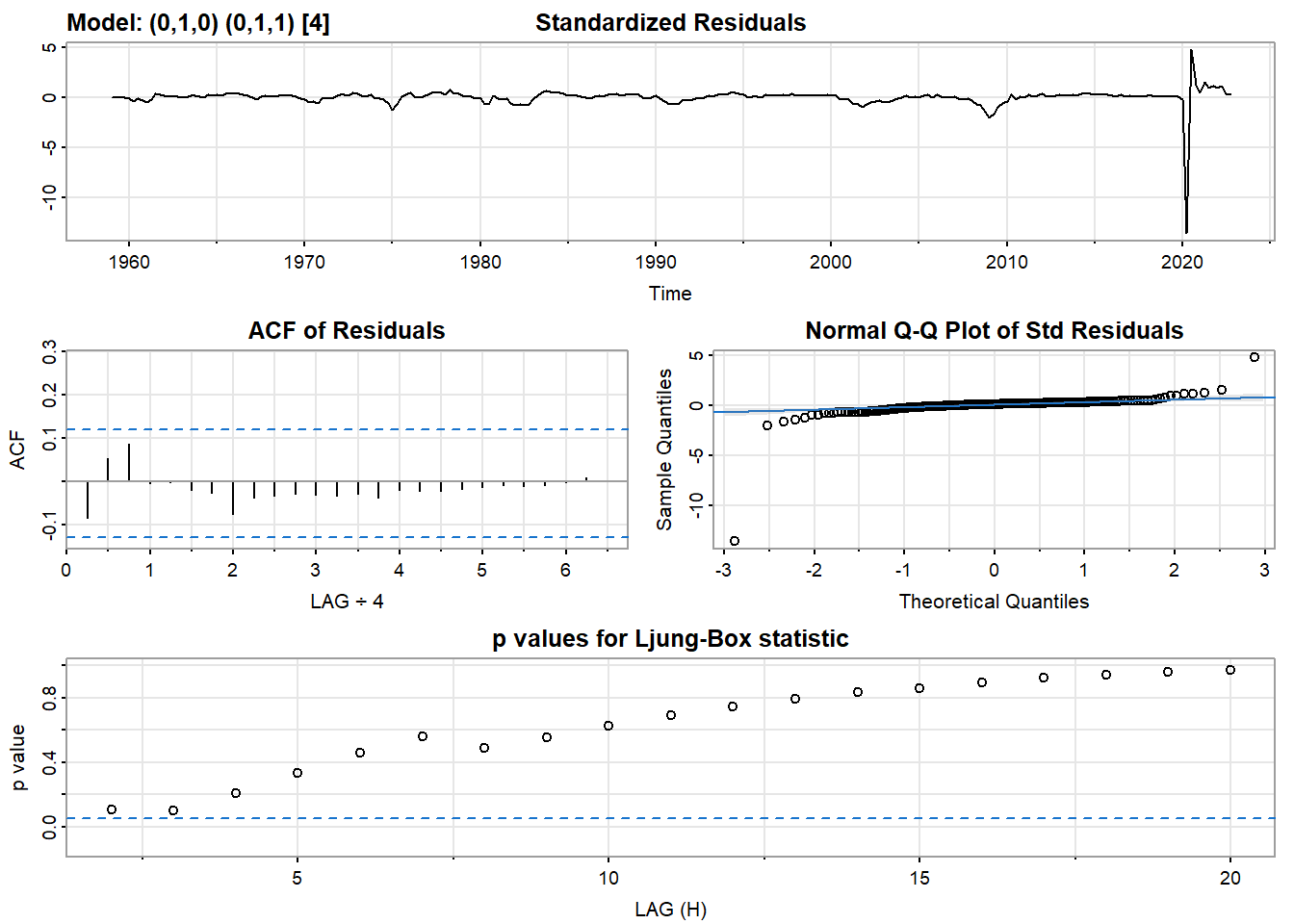
Show the code
cat(model_output[21:50], model_output[length(model_output)], sep = "\n")$fit
Call:
arima(x = xdata, order = c(p, d, q), seasonal = list(order = c(P, D, Q), period = S),
include.mean = !no.constant, transform.pars = trans, fixed = fixed, optim.control = list(trace = trc,
REPORT = 1, reltol = tol))
Coefficients:
sma1
-0.9492
s.e. 0.0345
sigma^2 estimated as 1852941: log likelihood = -2172.03, aic = 4348.06
$degrees_of_freedom
[1] 250
$ttable
Estimate SE t.value p.value
sma1 -0.9492 0.0345 -27.4916 0
$AIC
[1] 17.32293
$AICc
[1] 17.32299
$BIC
[1] 17.35102Model Fitting
Show the code
fit <- Arima(gdp_ts, order=c(0,1,0), seasonal=c(0,1,1))
summary(fit)
Series: gdp_ts
ARIMA(0,1,0)(0,1,1)[4]
Coefficients:
sma1
-0.9492
s.e. 0.0345
sigma^2 = 1860405: log likelihood = -2172.03
AIC=4348.06 AICc=4348.1 BIC=4355.11
Training set error measures:
ME RMSE MAE MPE MAPE MASE
Training set 3.482494 1347.888 492.0962 0.0137906 0.4616182 0.2031885
ACF1
Training set -0.08526289forecasting
Show the code
fit %>% forecast(h=12) %>% autoplot() #next 3 years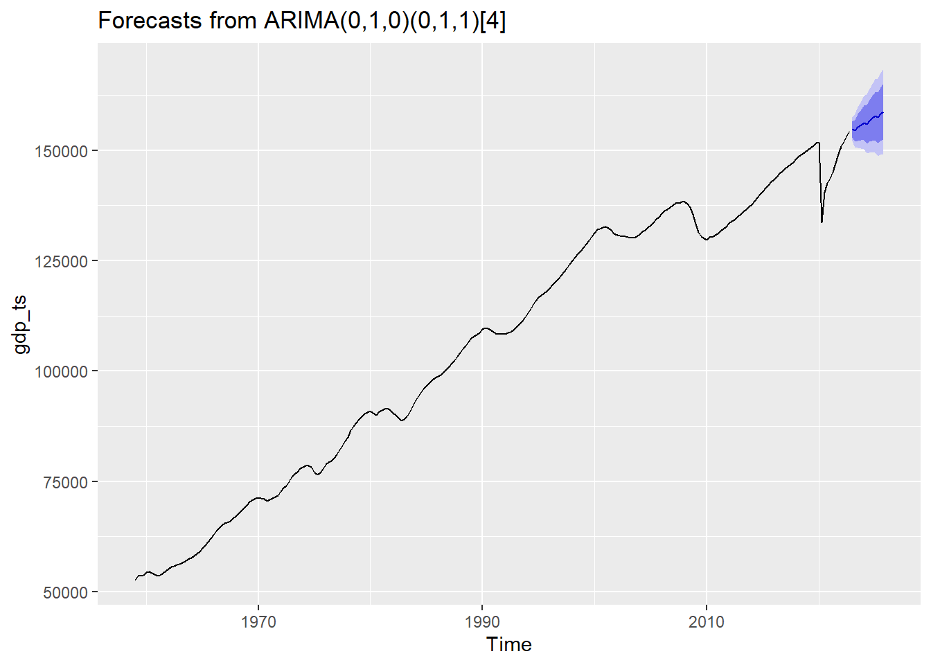
Show the code
sarima.for(gdp_ts, 12, 0,1,0,0,1,1,4)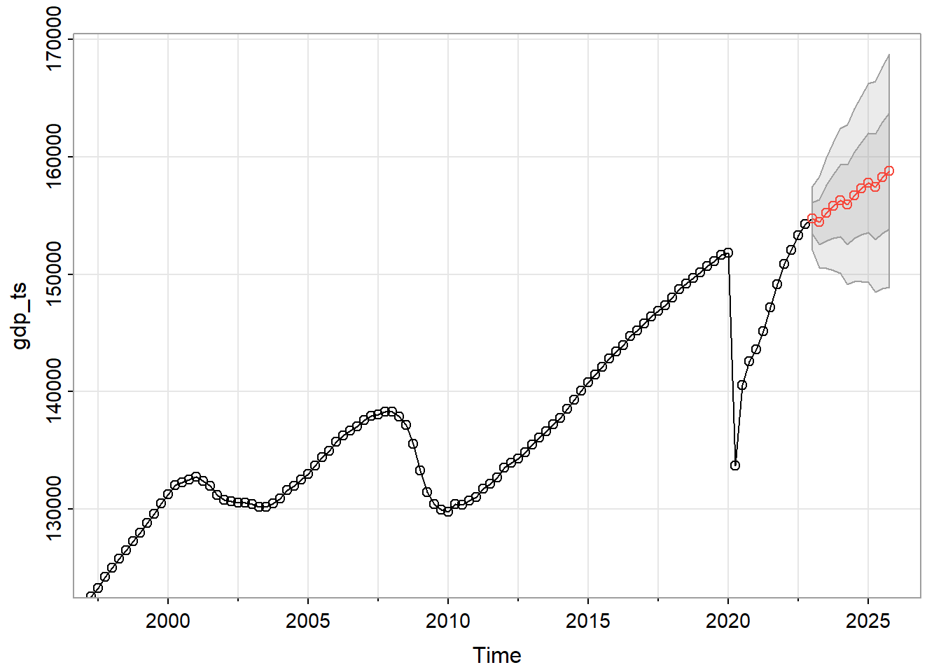
$pred
         Qtr1     Qtr2     Qtr3     Qtr4
2023 154768.4 154437.3 155221.5 155790.7
2024 156273.1 155942.0 156726.2 157295.5
2025 157777.8 157446.7 158231.0 158800.2

$se
         Qtr1     Qtr2     Qtr3     Qtr4
2023 1361.322 1925.194 2357.869 2722.631
2024 3075.622 3392.066 3681.408 3949.611
2025 4224.838 4483.186 4727.437 4959.674
Compare with Benchmark methods
Show the code
fit <- Arima(gdp_ts, order=c(0,1,0), seasonal=c(0,1,1))

autoplot(gdp_ts) +
  autolayer(meanf(gdp_ts, h=12),
            series="Mean", PI=FALSE) +
  autolayer(naive(gdp_ts, h=12),
            series="Naïve", PI=FALSE) +
  autolayer(snaive(gdp_ts, h=12),
            series="SNaïve", PI=FALSE)+
  autolayer(rwf(gdp_ts, h=12, drift=TRUE),
            series="Drift", PI=FALSE)+
  autolayer(forecast(fit,12),
            series="fit",PI=FALSE) +
  guides(colour=guide_legend(title="Forecast"))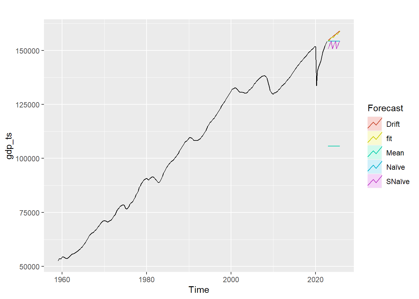
Show the code
f2 <- snaive(gdp_ts, h=12)

accuracy(f2)
ME RMSE MAE MPE MAPE MASE ACF1
Training set 1575.474 3048.225 2421.87 1.628746 2.330202 1 0.7384914Show the code
summary(fit)Series: gdp_ts
ARIMA(0,1,0)(0,1,1)[4]
Coefficients:
sma1
-0.9492
s.e. 0.0345
sigma^2 = 1860405: log likelihood = -2172.03
AIC=4348.06 AICc=4348.1 BIC=4355.11
Training set error measures:
ME RMSE MAE MPE MAPE MASE
Training set 3.482494 1347.888 492.0962 0.0137906 0.4616182 0.2031885
ACF1
Training set -0.08526289Cross Validation
Show the code
k <- 75 # minimum data length for fitting a model  n*0.3
n <- length(gdp_ts)

i=1
err1 = c()
#err2 = c()

for(i in 1:(n-k))
{
  xtrain <- gdp_ts[1:(k-1)+i] #observations from 1 to 75
  xtest <- gdp_ts[k+i] #76th observation as the test set

  # Arima(gdp_ts, order=c(0,1,0), seasonal=c(0,1,1))
  fit <- Arima(xtrain, order=c(0,1,0), seasonal=c(0,1,1),include.drift=FALSE, method="ML")
  fcast1 <- forecast(fit, h=1)

  #capture error for each iteration
  # This is mean absolute error
  err1 = c(err1, abs(fcast1$mean-xtest))
  #err2 = c(err2, abs(fcast2$mean-xtest))

  # This is mean squared error
  err3 = c(err1, (fcast1$mean-xtest)^2)
  #err4 = c(err2, (fcast2$mean-xtest)^2)

}

(MAE1=mean(err1)) # This is mean absolute error
[1] 771.8619Show the code
MSE1=mean(err1)
MSE1
[1] 771.8619