ARMA/ARIMA/SARIMA Models for LLY
Step 1: Determine the stationality of time series
Stationality is a pre-requirement of training ARIMA model. This is because term ‘Auto Regressive’ in ARIMA means it is a linear regression model that uses its own lags as predictors, which work best when the predictors are not correlated and are independent of each other. Stationary time series make sure the statistical properties of time series do not change over time.
Based on information obtained from both ACF graphs and Augmented Dickey-Fuller Test, the time series data is non-stationary.
Show the code
LLY_acf <- ggAcf(LLY_ts,100)+ggtitle("LLY ACF Plot")

LLY_pacf <- ggPacf(LLY_ts,100)+ggtitle("PACF Plot for UHNs")
grid.arrange(LLY_acf, LLY_pacf,nrow=2)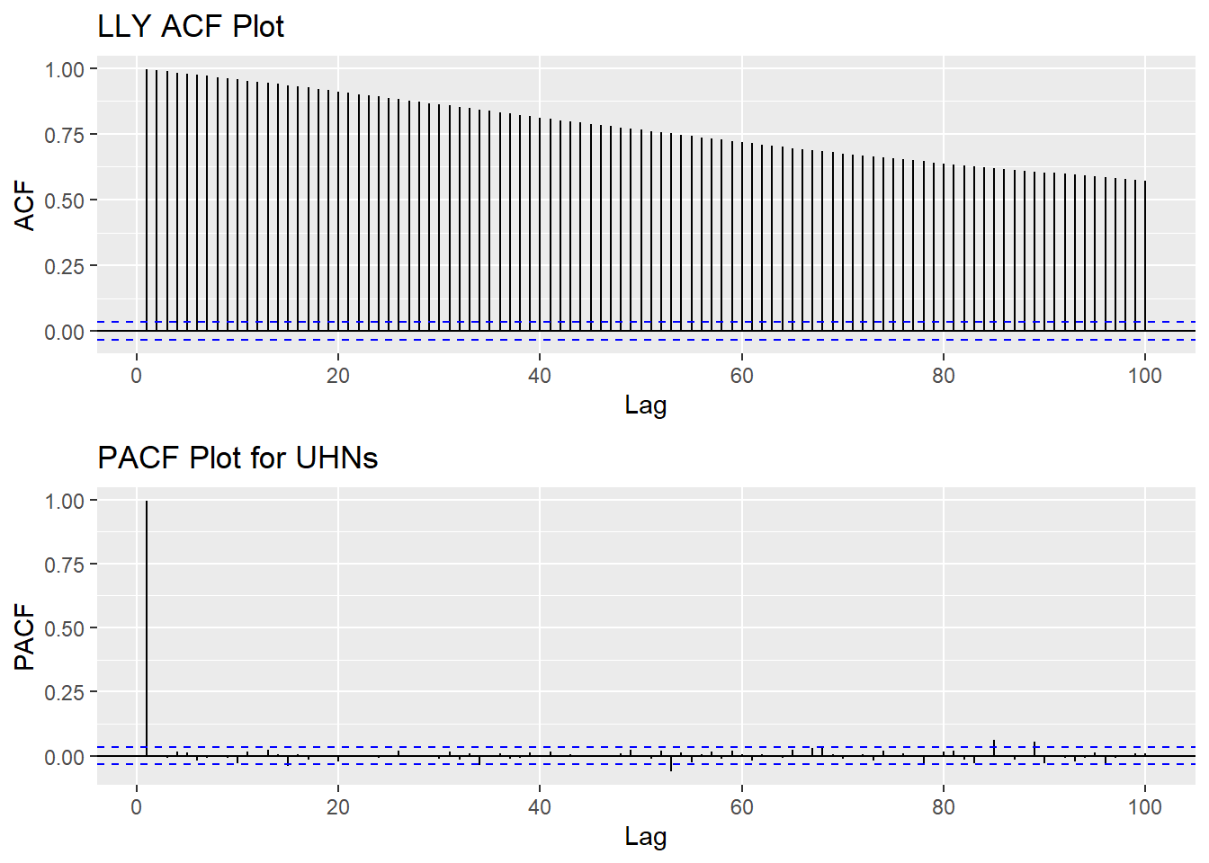
Show the code
tseries::adf.test(LLY_ts)
    Augmented Dickey-Fuller Test

data:  LLY_ts
Dickey-Fuller = -2.8006, Lag order = 14, p-value = 0.2393
alternative hypothesis: stationary
Step 2: Eliminate Non-Stationality
Since this data is non-stationary, it is important to necessary to convert it to stationary time series. This step employs a series of actions to eliminate non-stationality, i.e. differencing the data. It turns out the 1st differened data has shown good stationary property, there are no need to go further at 2nd differencing. What is more, the Augmented Dickey-Fuller Test also confirmed that the 1st differenced data is stationary. Therefore, the1st differencing would be the actions taken to eliminate the non-stationality.
Show the code
plot1<- ggAcf((LLY_ts) %>%diff(), 50, main="ACF Plot for 1st differenced Data")
plot2<- ggAcf((LLY_ts) %>%diff()%>%diff(),50, main="ACF Plot for 2nd differenced Data")

grid.arrange(plot1, plot2,nrow=2)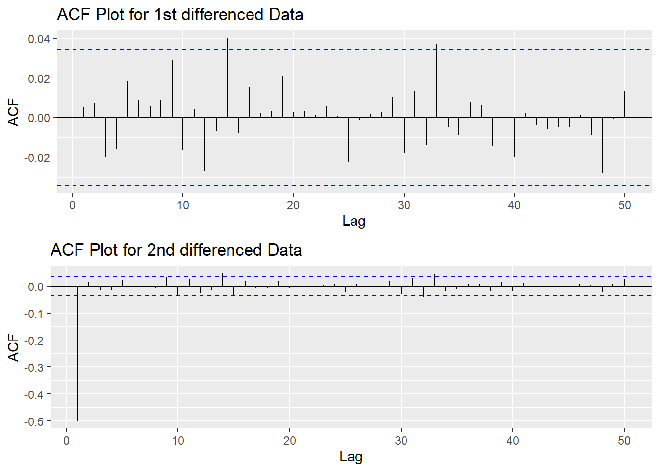
Show the code
tseries::adf.test((LLY_ts) %>%diff())
    Augmented Dickey-Fuller Test

data:  (LLY_ts) %>% diff()
Dickey-Fuller = -14.381, Lag order = 14, p-value = 0.01
alternative hypothesis: stationary
Step 3: Determine p,d,q Parameters
The standard notation of ARIMA(p,d,q) include p,d,q 3 parameters. Here are the representations: - p: The number of lag observations included in the model, also called the lag order; order of the AR term. - d: The number of times that the raw observations are differenced, also called the degree of differencing; number of differencing required to make the time series stationary. - q: order of moving average; order of the MA term. It refers to the number of lagged forecast errors that should go into the ARIMA Model.
Show the code
plot3<- ggPacf((LLY_ts) %>%diff(),50, main="PACF Plot for Log Transformed & 1st differenced Data")

grid.arrange(plot1,plot3)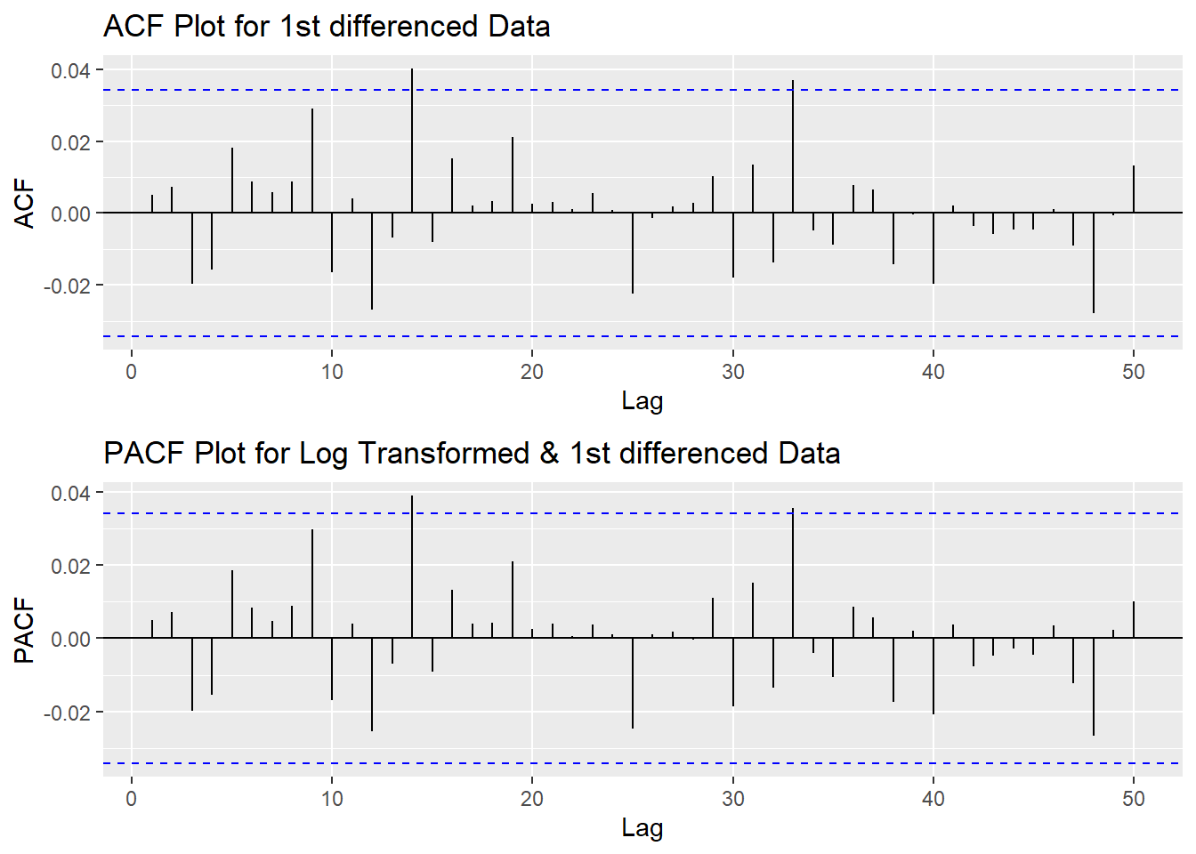
According to the PACF plot and ACF plot above, there are no significant peaks on both graph, therefore, here set both p and q as 0. Since I only differenced the data once, the d would be 1.
Step 4: Fit ARIMA(p,d,q) model
Show the code
fit1 <- Arima((LLY_ts), order=c(0, 1, 0),include.drift = TRUE)
summary(fit1)
Series: (LLY_ts)
ARIMA(0,1,0) with drift
Coefficients:
drift
0.0183
s.e. 0.1283
sigma^2 = 53.71: log likelihood = -11128.73
AIC=22261.47 AICc=22261.47 BIC=22273.65
Training set error measures:
ME RMSE MAE MPE MAPE MASE
Training set 2.349624e-05 7.326456 2.206738 -0.1331229 1.443189 0.02767164
ACF1
Training set 0.004971149Model Diagnostics
- Inspection of the time plot of the standardized residuals below shows no obvious patterns.
- Notice that there may be outliers, with a few values exceeding 3 standard deviations in magnitude.
- The ACF of the standardized residuals shows no apparent departure from the model assumptions, no significant lags shown.
- The normal Q-Q plot of the residuals shows that the assumption of normality is reasonable, with the exception of the fat-tailed.
- The model appears to fit well.
Show the code
model_output <- capture.output(sarima((LLY_ts), 0,1,0))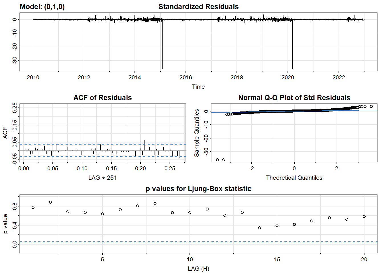
Show the code
cat(model_output[9:37], model_output[length(model_output)], sep = "\n") #to get rid of the convergence status and details of the optimization algorithm used by the sarima() $fit
Call:
arima(x = xdata, order = c(p, d, q), seasonal = list(order = c(P, D, Q), period = S),
xreg = constant, transform.pars = trans, fixed = fixed, optim.control = list(trace = trc,
REPORT = 1, reltol = tol))
Coefficients:
constant
0.0183
s.e. 0.1283
sigma^2 estimated as 53.69: log likelihood = -11128.73, aic = 22261.47
$degrees_of_freedom
[1] 3262
$ttable
Estimate SE t.value p.value
constant 0.0183 0.1283 0.143 0.8863
$AIC
[1] 6.822393
$AICc
[1] 6.822394
$BIC
[1] 6.826126Compare with auto.arima() function
auto.arima() returns best ARIMA model according to either AIC, AICc or BIC value. The function conducts a search over possible model within the order constraints provided. The parameters matches with the model.
Show the code
auto.arima((LLY_ts))Series: (LLY_ts)
ARIMA(0,1,0)
sigma^2 = 53.69: log likelihood = -11128.74
AIC=22259.49 AICc=22259.49 BIC=22265.58Step 5: Forecast
The blue part in graph below forecast the next 100 values of LLY stock price in 80% and 95% confidence level.
Show the code
LLY_ts %>%
  Arima(order=c(0,1,0),include.drift = TRUE) %>%
  forecast(100) %>%
  autoplot() +
  ylab("LLY stock prices prediction") + xlab("Year")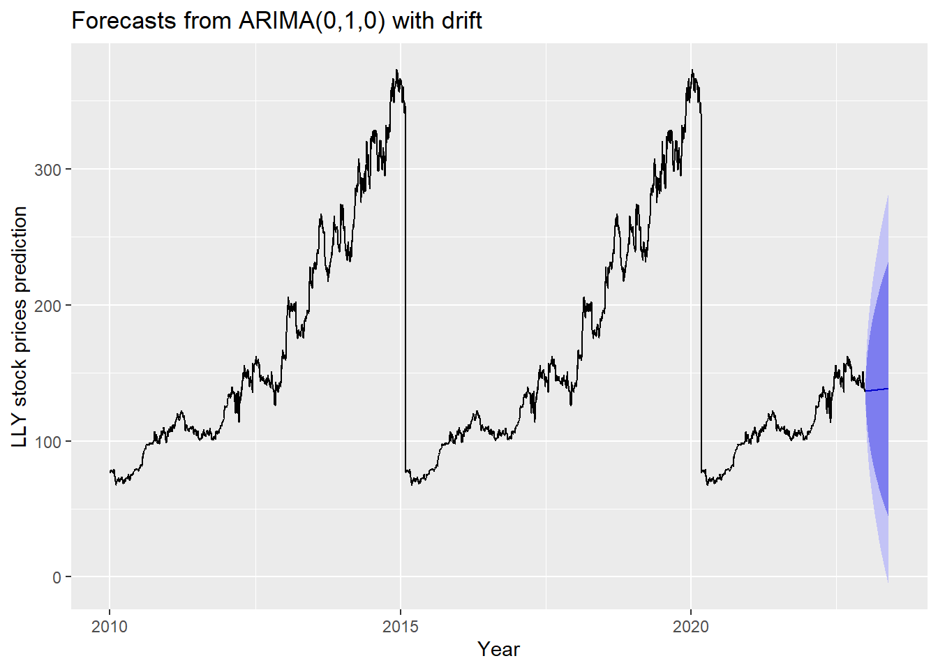
Step 6: Compare ARIMA model with the benchmark methods
Forecasting benchmarks are very important when testing new forecasting methods, to see how well they perform against some simple alternatives.
Average method
Here, the forecast of all future values are equal to the average of the historical data. The residual plot of this method is not stationary.
Show the code
f1<-meanf((LLY_ts), h=251) #mean
#summary(f1)
checkresiduals(f1)#serial correlation ; Lung Box p <0.05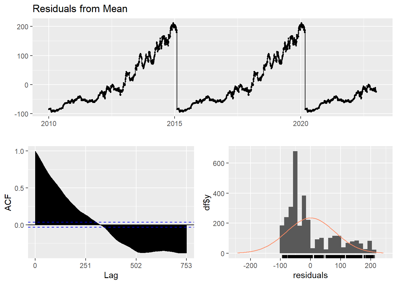
    Ljung-Box test

data:  Residuals from Mean
Q* = 300420, df = 501, p-value < 2.2e-16

Model df: 1.   Total lags used: 502
Naive method
This method simply set all forecasts to be the value of the last observation. According to error measurement here, ARIMA(4,1,3) outperform the average method.
Show the code
f2<-naive((LLY_ts), h=11) # naive method
summary(f2)
Forecast method: Naive method

Model Information:
Call: naive(y = (LLY_ts), h = 11)

Residual sd: 7.3276

Error measures:
                     ME     RMSE      MAE        MPE     MAPE       MASE
Training set 0.01834098 7.327602 2.208937 -0.1191376 1.444964 0.02769921
                    ACF1
Training set 0.004970975

Forecasts:
         Point Forecast    Lo 80    Hi 80     Lo 95    Hi 95
2023.004       136.5567 127.1660 145.9474 122.19488 150.9186
2023.008       136.5567 123.2763 149.8372 116.24601 156.8674
2023.012       136.5567 120.2915 152.8219 111.68129 161.4321
2023.016       136.5567 117.7753 155.3381 107.83305 165.2804
2023.020       136.5567 115.5585 157.5550 104.44268 168.6708
2023.024       136.5567 113.5543 159.5591 101.37755 171.7359
2023.028       136.5567 111.7113 161.4022  98.55887 174.5546
2023.032       136.5567 109.9958 163.1176  95.93531 177.1781
2023.036       136.5567 108.3846 164.7288  93.47121 179.6422
2023.040       136.5567 106.8607 166.2527  91.14061 181.9728
2023.044       136.5567 105.4113 167.7021  88.92390 184.1895
Show the code
checkresiduals(f2)#serial correlation ; Lung Box p <0.05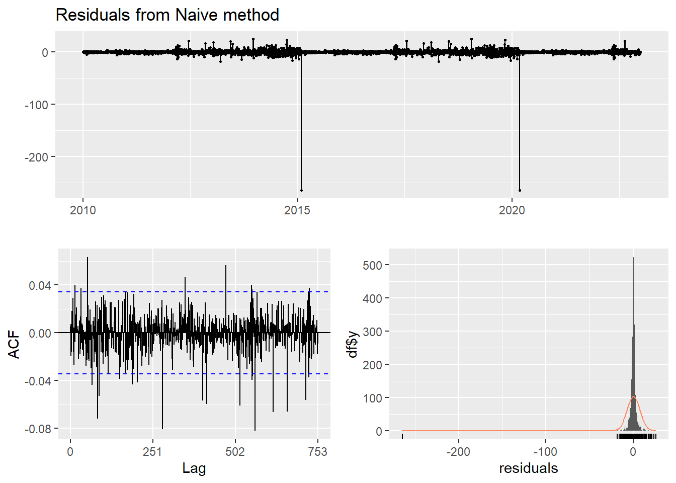
    Ljung-Box test

data:  Residuals from Naive method
Q* = 438.09, df = 502, p-value = 0.9816

Model df: 0.   Total lags used: 502
Seasonal naive method
This method is useful for highly seasonal data, which can set each forecast to be equal to the last observed value from the same season of the year. Here seasonal naive is used to forecast the next 4 values for the LLY stock price series.
Show the code
f3<-snaive((LLY_ts), h=4) #seasonal naive method
summary(f3)
Forecast method: Seasonal naive method

Model Information:
Call: snaive(y = (LLY_ts), h = 4)

Residual sd: 108.2255

Error measures:
                   ME     RMSE      MAE       MPE     MAPE MASE      ACF1
Training set 4.249799 108.2255 79.74729 -23.12158 65.75914    1 0.9950134

Forecasts:
         Point Forecast     Lo 80    Hi 80     Lo 95    Hi 95
2023.004       105.4368 -33.25979 244.1334 -106.6813 317.5550
2023.008       106.4282 -32.26840 245.1248 -105.6899 318.5464
2023.012       107.5895 -31.10708 246.2861 -104.5286 319.7077
2023.016       106.2299 -32.46667 244.9265 -105.8882 318.3481
Show the code
checkresiduals(f3) #serial correlation ; Lung Box p <0.05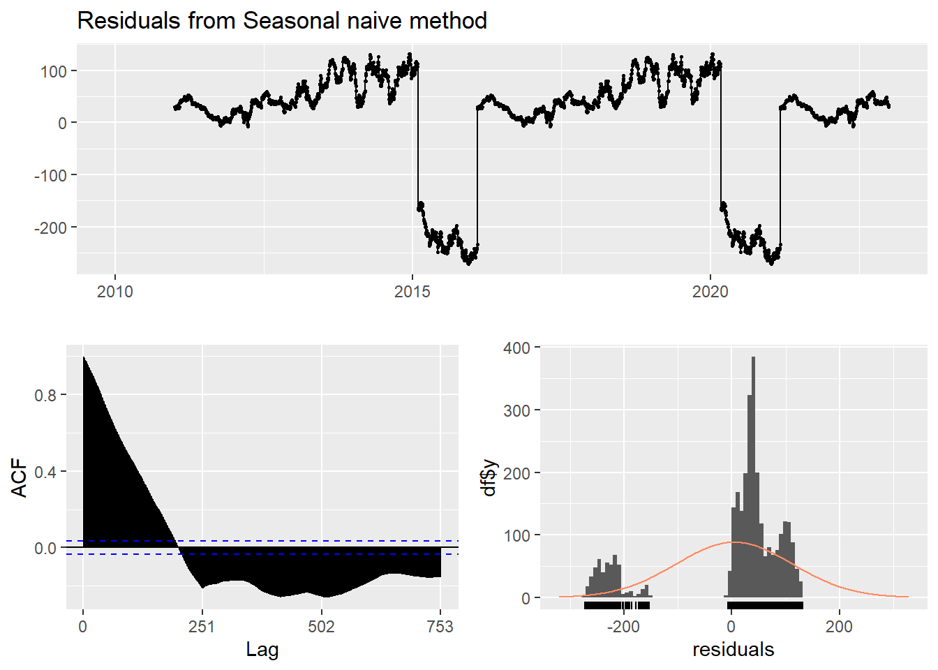
    Ljung-Box test

data:  Residuals from Seasonal naive method
Q* = 235237, df = 502, p-value < 2.2e-16

Model df: 0.   Total lags used: 502
Drift Method
A variation on the naïve method is to allow the forecasts to increase or decrease over time, where the amount of change over time is set to be the average change seen in the historical data.
Show the code
f4 <- rwf((LLY_ts),drift=TRUE, h=20)
summary(f4)
Forecast method: Random walk with drift

Model Information:
Call: rwf(y = (LLY_ts), h = 20, drift = TRUE)

Drift: 0.0183  (se 0.1283)
Residual sd: 7.3287

Error measures:
                       ME     RMSE      MAE        MPE     MAPE       MASE
Training set 5.431461e-15 7.327579 2.207391 -0.1331943 1.443601 0.02767983
                    ACF1
Training set 0.004970975

Forecasts:
         Point Forecast     Lo 80    Hi 80     Lo 95    Hi 95
2023.004       136.5751 127.18151 145.9686 122.20887 150.9413
2023.008       136.5934 123.30688 149.8799 116.27342 156.9134
2023.012       136.6117 120.33665 152.8868 111.72114 161.5023
2023.016       136.6301 117.83435 155.4258 107.88449 165.3757
2023.020       136.6484 115.63094 157.6659 104.50496 168.7919
2023.024       136.6668 113.63975 159.6938 101.44998 171.8835
2023.028       136.6851 111.80928 161.5609  98.64081 174.7294
2023.032       136.7034 110.10600 163.3009  96.02617 177.3807
2023.036       136.7218 108.50663 164.9369  93.57042 179.8731
2023.040       136.7401 106.99419 166.4861  91.24765 182.2326
2023.044       136.7585 105.55590 167.9610  89.03826 184.4787
2023.048       136.7768 104.18182 169.3718  86.92707 186.6265
2023.052       136.7951 102.86403 170.7263  84.90198 188.6883
2023.056       136.8135 101.59613 172.0309  82.95318 190.6738
2023.060       136.8318 100.37284 173.2908  81.07261 192.5911
2023.064       136.8502  99.18974 174.5106  79.25351 194.4468
2023.068       136.8685  98.04311 175.6939  77.49018 196.2468
2023.072       136.8869  96.92975 176.8440  75.77774 197.9960
2023.076       136.9052  95.84692 177.9635  74.11198 199.6984
2023.080       136.9235  94.79222 179.0549  72.48925 201.3578
Show the code
checkresiduals(f4)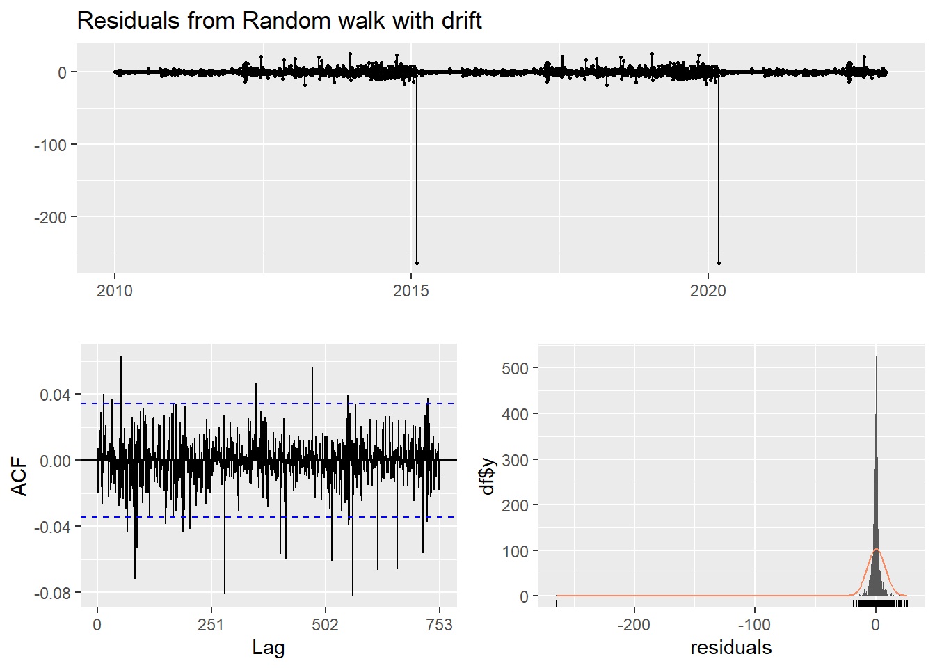
    Ljung-Box test

data:  Residuals from Random walk with drift
Q* = 438.09, df = 501, p-value = 0.9801

Model df: 1.   Total lags used: 502
Show the code
autoplot(LLY_ts) +
  autolayer(meanf(LLY_ts, h=100),
            series="Mean.tr", PI=FALSE) +
  autolayer(naive((LLY_ts), h=100),
            series="Naïve.tr", PI=FALSE) +
  autolayer(rwf((LLY_ts), drift=TRUE, h=100),
            series="Drift.tr", PI=FALSE) +
  autolayer(forecast(fit1,100),
            series="fit",PI=FALSE) +
  ggtitle("LLY Stock Price") +
  xlab("Time") + ylab("Price") +
  guides(colour=guide_legend(title="Forecast"))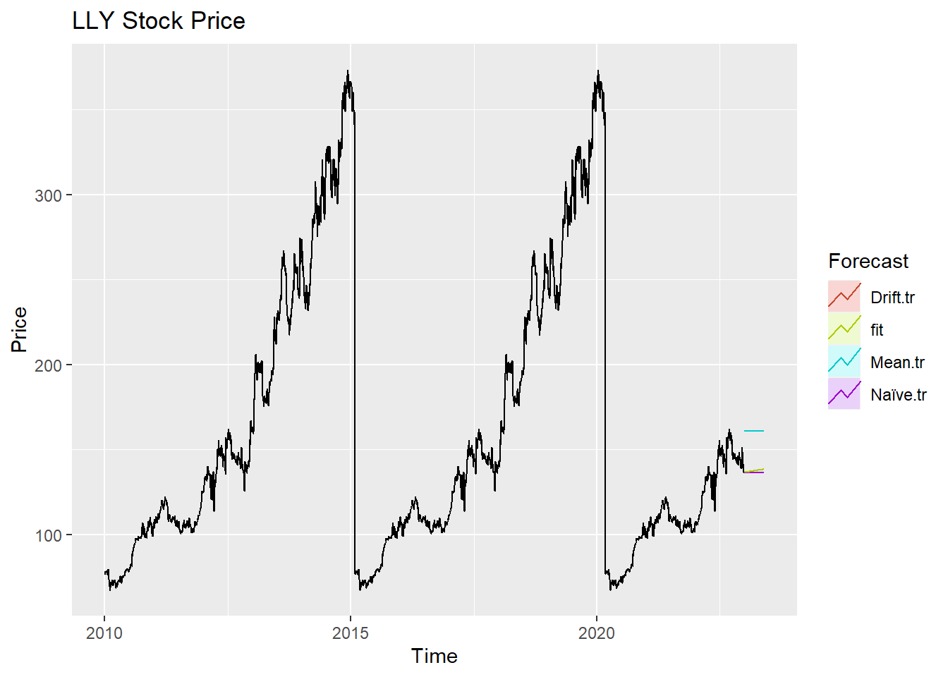
According to the graph above, ARIMA(0,1,0) outperform most of benchmark method, though its performance is very similar to drift method.